

LoCoH Parameter Explorer
Summary
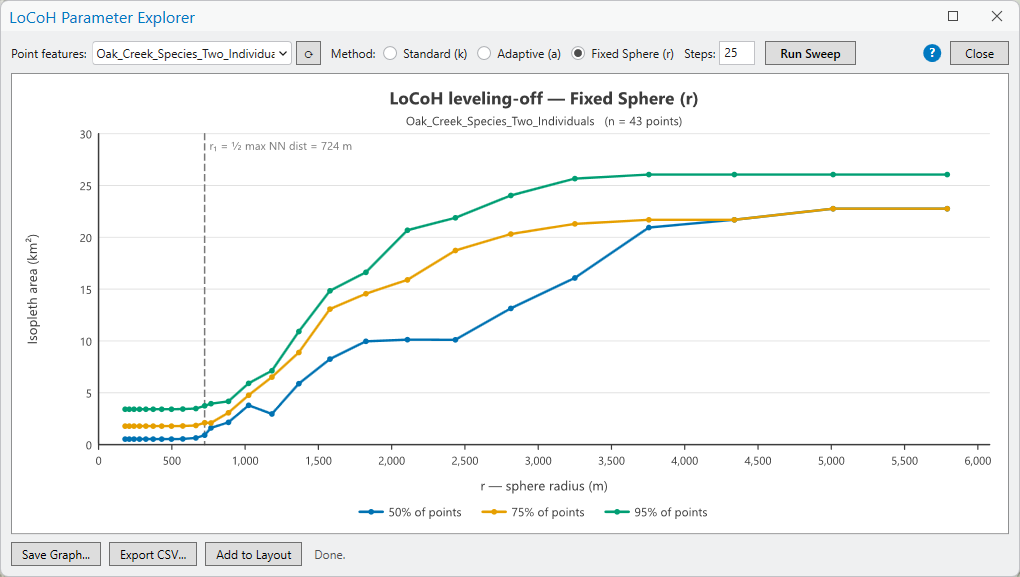
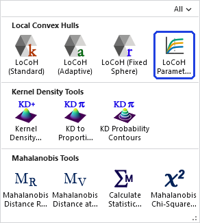
An interactive window that runs the Getz et al. (2007) leveling-off analysis for choosing a LoCoH parameter: pick a point feature class, choose the Standard (k), Adaptive (a) or Fixed Sphere (r) method, and the window sweeps the parameter across a sequence of values, building the local hulls at every value and charting the areas of the 50%, 75% and 95% isopleths against it. A dashed line marks the starting value the method's authors recommend — a rule of thumb computed from your own data (k = √n for the Standard method, for example) that gives the search a sensible first anchor. Where the curves climb, holes are filling; where they flatten, the estimate is stable; where they jump, hulls have begun to bridge a real gap. Run it before committing to a parameter in the LoCoH tools; this tool may help you choose an appropriate LoCoH sizing parameter value. Export the chart (PNG/SVG), the sweep table (CSV), or place the chart on a layout.
Why sweep the parameter?
Every LoCoH variant has one governing parameter, and the choice matters more than any other decision in the analysis: too small fragments the range with spurious holes, too large inflates it toward the minimum convex polygon. The LoCoH literature's advice is empirical — build hull sets across a range of values and watch how the isopleth areas respond (Getz et al. 2007; Lyons et al. 2013) — which is exactly the tedious, repetitive work a tool should absorb. This window does the whole procedure in one click, on the very data you are about to analyze, with the layer's selection honored — so a season of multi-animal telemetry can be swept one animal at a time by selecting each animal's locations.
Reading the curves
Each curve tracks one isopleth — the cumulative-hull polygon that first encloses 50%, 75% or 95% of the locations — and the horizontal axis is the swept parameter. Three behaviors carry the meaning:
Climbing — as the parameter grows, hulls widen and spurious holes fill; the isopleth areas rise quickly. Flattening — when the artifacts are gone, adding more neighbors changes little; a plateau is the signature of a stable estimate, and the value at its start is the minimum spurious hole covering. Jumping — a sudden step up means the hulls just bridged a genuine gap: a hole or bay the animal truly avoided has been swallowed. Treat the value just before a jump as a ceiling.
No prior estimate of the true home-range area is needed — the judgment reads the shape of the curves plus your own knowledge of which gaps are real. And it is honest to say the judgment is a skill: as Getz et al. (2007) put it, “only experience with the method, however, will reveal appropriate methods for deciding when this leveling off has been achieved.” This window exists to make that experience cheap to acquire.
The three sweeps, one dataset
The charts below sweep the same data — the two-individual Oak Creek dataset from the Concave Hull page, 43 locations in two clusters with a gap between them — through all three methods. The gap dominates every chart, and finding it in each is good practice in reading sweeps.
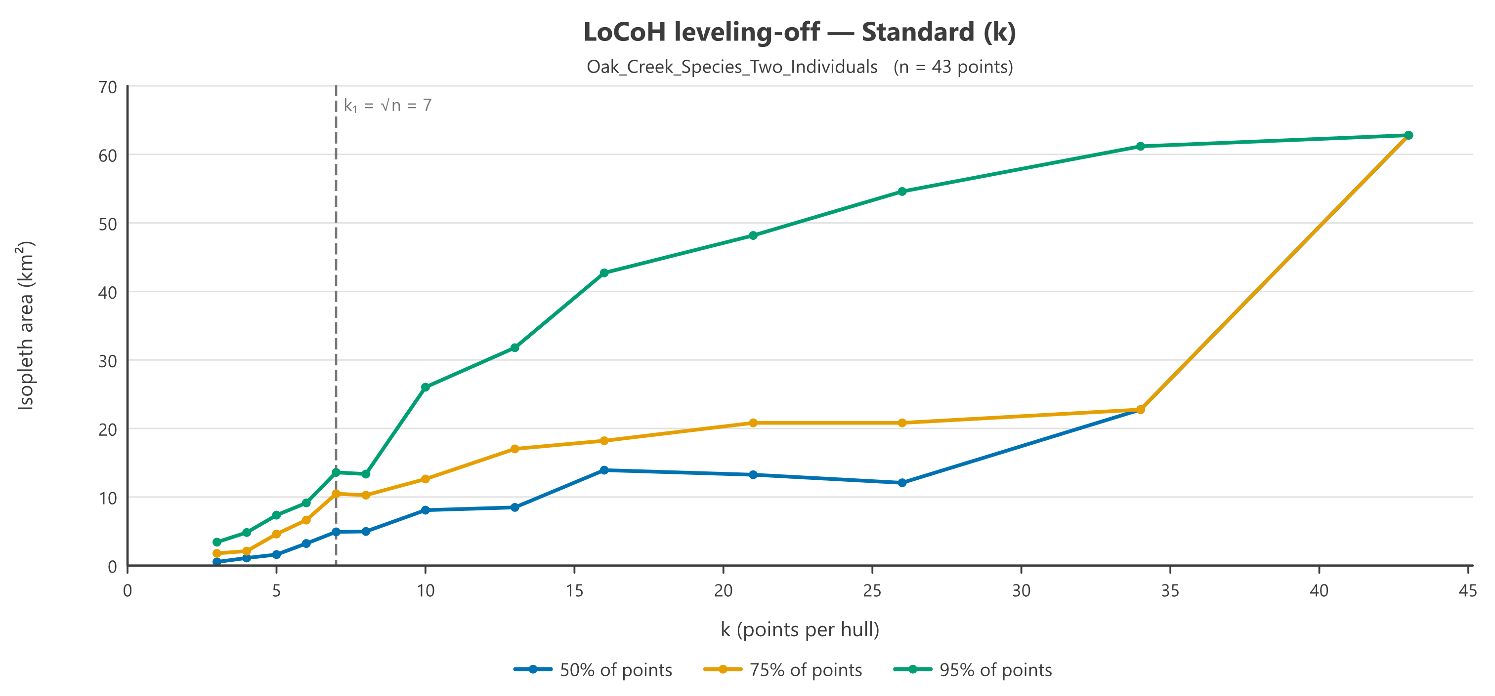
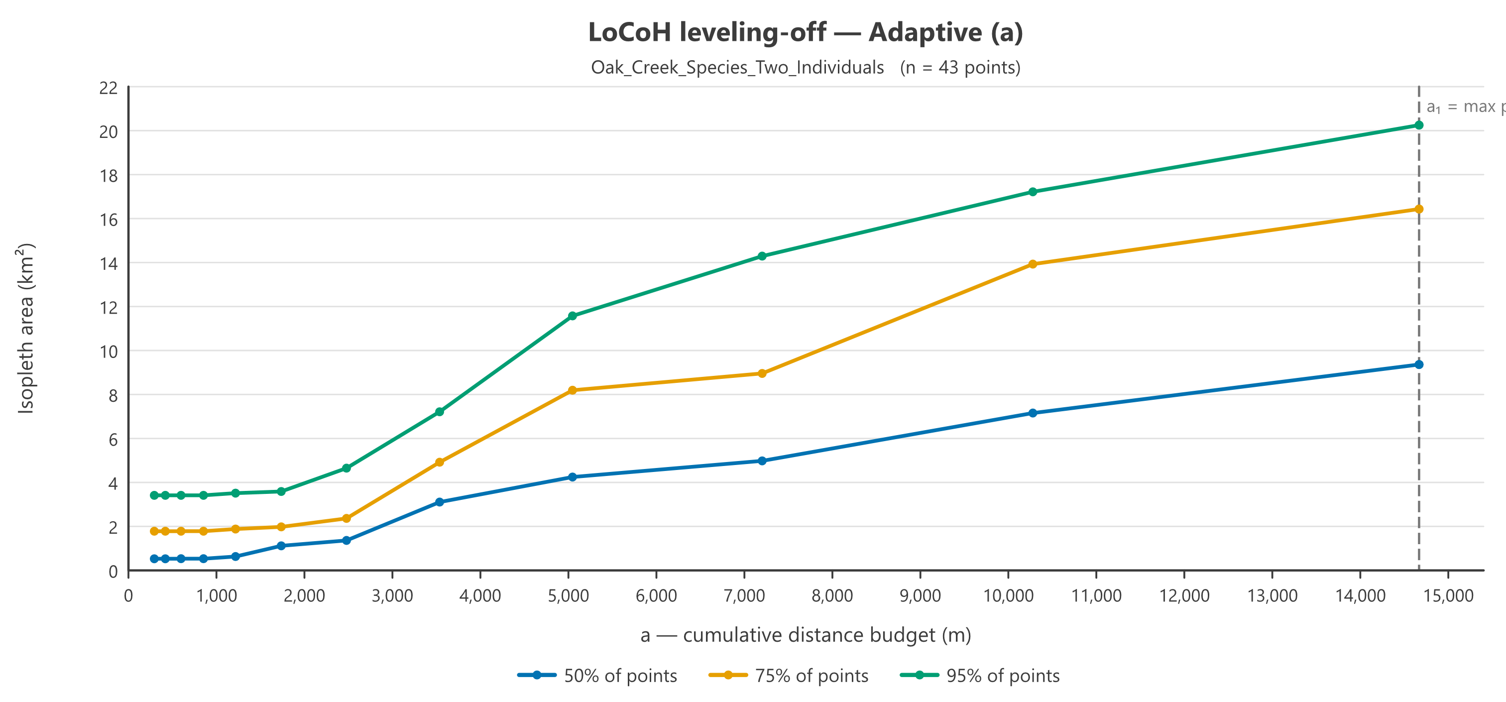
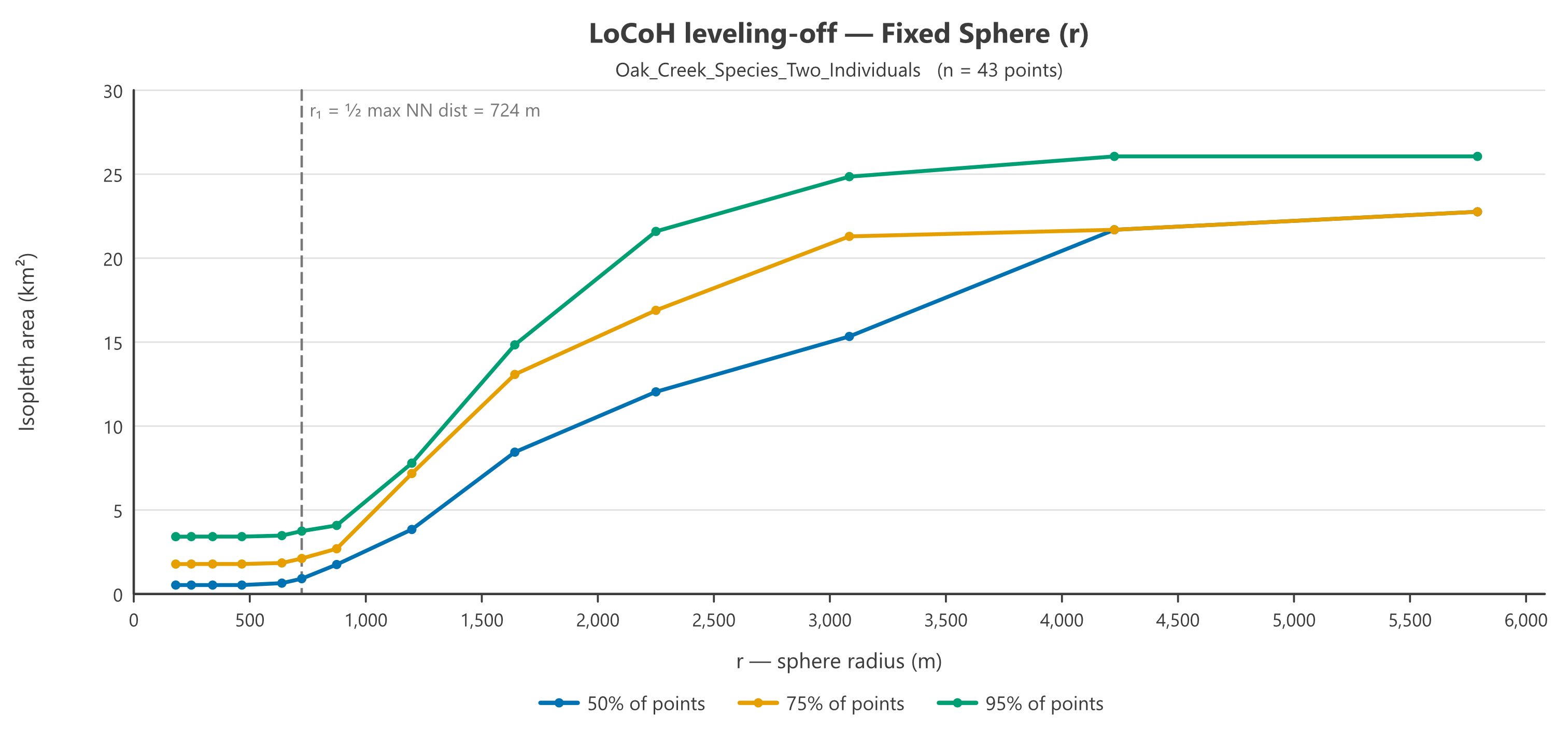
The common lesson: when a curve jumps, ask what geography just got bridged. On this dataset every jump is the gap between the two individuals — a warning that no single parameter honestly describes both animals at once. The remedies are the ones the charts suggest: keep the parameter below the jump, or better, sweep and analyze each animal separately (select one animal's locations and re-run; the selection is honored).
From sweep to home ranges
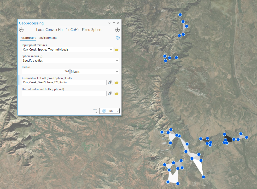
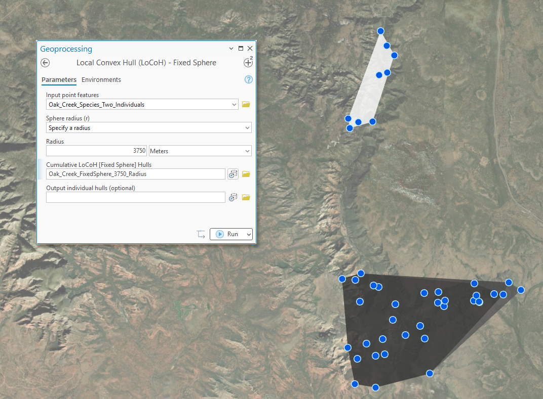
The payoff comes when the curves send you back to the LoCoH tools with actual numbers. The Fixed Sphere sweep above picked out two good plateaus: one right at the heuristic, r = 724 m, and a second at about r = 3,750 m, where the gaps had finished filling in. So we ran the LoCoH (Fixed Sphere) tool twice, once at each radius — and now we can choose between two defensible home-range estimates, each answering its own question. Possibly the 724 m version serves to identify the core areas, while the 3,750 m version is more the general home range.
A tour of the window
Pick the point features, choose the method, optionally adjust Steps (how many parameter values to try, 4–40; more steps draw smoother curves and take proportionally longer), and click Run Sweep. A progress bar tracks the hull building, and Cancel stops a long sweep. The sweep values are spaced logarithmically from very tight to each method's natural ceiling — k up to n, a up to the maximum pairwise distance, r to several times the heuristic — with the heuristic value itself always included, so the dashed line always touches a computed point. Geographic (latitude–longitude) points are handled in a data-centered equal-area projection, and areas are always square kilometers.
Save Graph... exports the chart as a 300-dpi PNG or scalable SVG; Export CSV... writes the sweep table (parameter value and the three isopleth areas per row); Add to Layout places the chart on a layout as native, individually editable graphic elements — the active layout when one is open, otherwise you pick from the project's layouts. The blue ? opens this page.
Recommended citation
Credits and references
By Jeff Jenness, Jenness Enterprises (www.jennessent.com). The leveling-off analysis follows Getz et al. (2007); the isopleth-area-curve procedure follows the T-LoCoH practice of Lyons, Turner and Getz (2013).
- Getz, W. M., S. Fortmann-Roe, P. C. Cross, A. J. Lyons, S. J. Ryan, and C. C. Wilmers. 2007. LoCoH: nonparametric kernel methods for constructing home ranges and utilization distributions. PLoS ONE 2(2):e207. doi.org/10.1371/journal.pone.0000207
- Lyons, A. J., W. C. Turner, and W. M. Getz. 2013. Home range plus: a space-time characterization of movement over real landscapes. Movement Ecology 1:2. doi.org/10.1186/2051-3933-1-2
Licensing information
Works at every ArcGIS Pro license level (Basic, Standard, Advanced). No extension licenses are required.
Related tools and pages
- About LoCoH home-range analysis — the theory behind the curves.
- LoCoH (Standard), LoCoH (Adaptive), and LoCoH (Fixed Sphere) — the tools whose parameter this window chooses.