Concave Hull

Geometric Tools · geoprocessing tool · by Jeff Jenness

Works at every ArcGIS Pro license level

Summary

Builds a concave hull — the shape of a cloud of points — by any of the three classic methods: chi (characteristic) shapes, always one simple polygon containing every point; alpha shapes, the only method that can return multiple parts and interior holes; or the k-nearest-neighbours hull. One Concavity setting (0 = the convex hull, 100 = maximum detail, blank = automatic) controls how tightly the hull follows the points; an optional case field builds one hull per group. Equivalent to the concave-hull and alpha-shape tools of PostGIS, CGAL and QGIS; Esri's closest analog (Aggregate Points) needs an Advanced license.

The shape of a point cloud

The examples on this page follow a hypothetical canyon-dwelling species in Oak Creek Canyon, in northern Arizona. When the job is delineating a home range from a set of locations, the minimum convex polygon (MCP) — the convex hull — is often the first choice, and for a good reason: it is guaranteed to capture all the area the animal uses, along with every possible connector between locations. (Assuming good data, that is — all bets are off if you do not have a good sample of the animal's true range.) The MCP is conservative in exactly that sense: nothing the animal showed you is ever left outside.

The downside is that it sometimes captures far more territory than the animal uses, and the problem is most apparent with habitat specialists whose habitat occurs in distinct shapes on the landscape. Canyon-dwelling and riparian obligate species are the classic case: canyons and river systems are rarely shaped like a convex hull. They tend to be narrow and meandering, curving across the landscape in unpredictable directions — and the convex hull bridges straight across every bend, sweeping in areas the animal would obviously never use, like the plateau above the eastern edge of Oak Creek Canyon below. That is not just a cosmetic flaw: try to block that plateau off to protect the species, and anyone wanting to develop or do management work up there has a strong argument against you. The concave hull, on the other hand, follows the natural edges of the set of locations a lot better.

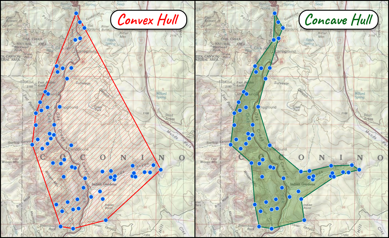
Two topographic maps of Oak Creek Canyon side by side, each with the same blue animal locations along the canyon. On the left, a red hatched convex hull bridges from the canyon across the plateau east of the rim, enclosing large areas with no locations at all. On the right, a green concave hull follows the canyon and its eastern side-canyon closely, keeping the plateau out — The same locations, two hulls. The convex hull (left) sweeps in the whole plateau above the canyon's eastern rim — country our canyon-dweller never touches. The concave hull (right) follows the canyon and its eastern arm the way the animal actually lives in them.

One caution before the details: a “concave hull” is a trickier object than it first sounds, because the problem has no single right answer. Taken to its logical extreme, the tightest possible concave boundary around a set of points degenerates into a spiderweb — threads of zero-width polygon connecting the points, technically containing them all and enclosing almost no area. This tool will not carve that far, but the lesson stands: there is a whole family of defensible shapes between the convex hull and the spiderweb, and you should expect to adjust the settings until the hull matches what you know about your species and your landscape.

Three methods, three lineages

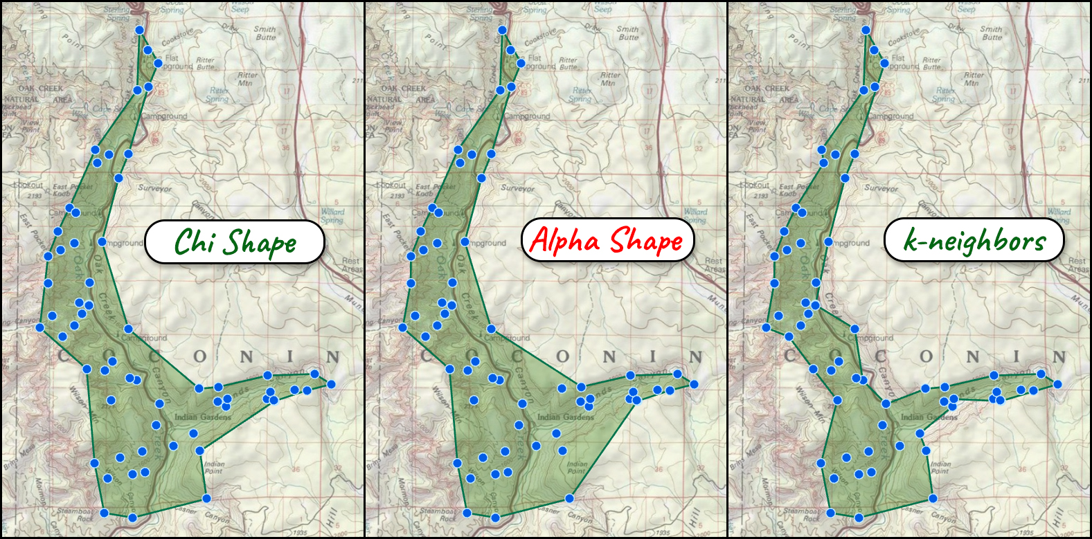
The three method choices are the three classic lineages of the concave-hull problem — genuinely different algorithms with different guarantees, not three flavors of one trick.

Chi shape (characteristic shape) — the default (Duckham, Kulik, Worboys and Galton 2008). Starts from the Delaunay triangulation, whose outer boundary is the convex hull, and repeatedly removes the longest boundary edge whenever removal keeps the shape clean. Its guarantees make it the best-behaved choice for most uses: always one simple polygon containing every point, degrading gracefully to the convex hull, with each tighter setting nested inside the last. Its Advanced parameter is the edge length threshold, a real distance: boundary edges longer than this are carved away, so a 500 m threshold means “no boundary segment may bridge a gap longer than 500 m.”

Alpha shape (Edelsbrunner, Kirkpatrick and Seidel 1983). Imagine erasing the plane with a disk of a chosen radius: the alpha shape is everything the disk cannot reach without hitting a point. This is the only method that can return multiple disjoint polygons and interior holes — two separate herds become two shapes, and telemetry ringing a lake keeps the lake as a hole (check Allow multiple parts and interior holes; leave it unchecked and the tool picks the smallest radius that keeps the shape in one piece). Its Advanced parameter is the alpha radius — the eraser disk's radius as a real distance: smaller disks reach into tighter bays and may drop outlying points entirely, larger disks approach the convex hull.

k-nearest-neighbours hull (Moreira and Santos 2007). A gift-wrapping walk around the cloud where each next boundary vertex is chosen among the current point's k nearest neighbours; smaller k hugs the points more tightly. If a walk fails to close around every point, the tool raises k automatically, settles on the smallest workable value, and reports the k it actually used in the output's K_used field. Its Advanced parameter is k itself: the number of neighbours each step of the walk may choose from. The Advanced section of the dialog shows the exact parameter for whichever method is chosen; giving one overrides the Concavity setting.

Three topographic maps of Oak Creek Canyon, each outlining the same dense set of animal locations: the chi shape, alpha shape, and k-neighbours hull, all three following the canyon closely with slightly different boundaries — The three methods on the full set of species locations, at their automatic settings. All three follow the canyon; the differences live in the details of how each lineage carves — and note that the k-neighbours hull does fine here, a point worth remembering when we revisit it below.

One Concavity setting

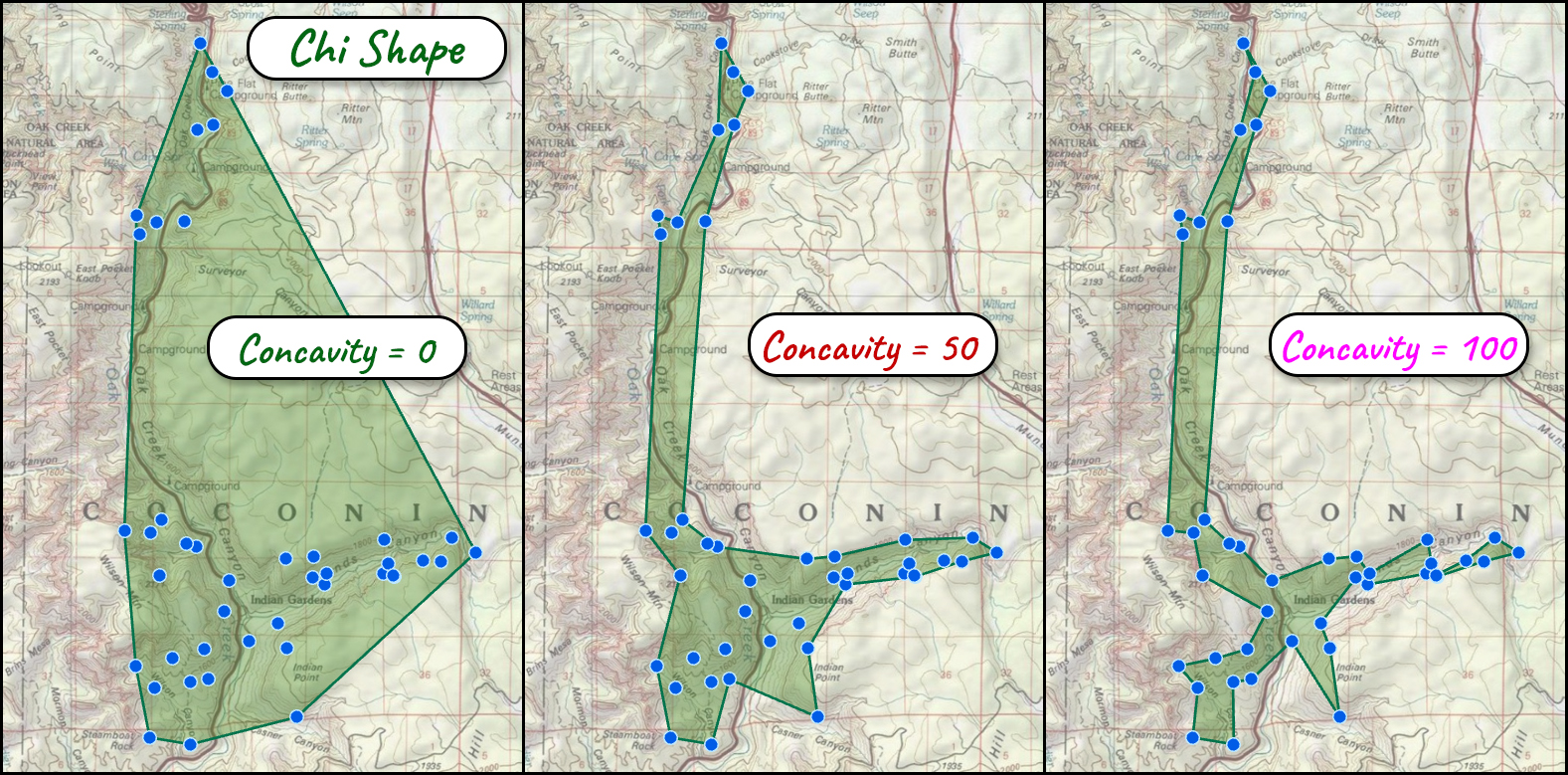
However different the machinery, all three methods answer to a single dial. Concavity runs from 0 — the convex hull, under every method — to 100, each method's true extreme: the exactly-covering alpha radius, the tightest k = 3, every removable chi edge gone. Left blank, each method picks its own automatic setting, and the automatics are deliberately more moderate than 100: the chi method separates gap-spanning edges from density-scale edges with a two-class threshold over its full nested family of shapes; the alpha method takes the smallest radius that keeps every point covered — the “optimal alpha” rule of CGAL and PostGIS — and then adds a 50% stability margin, because the exactly-covering radius tends toward spiky, one-triangle-wide isthmuses; the k-NN method uses a k that grows with the point count (about the square root of n). When you know the exact parameter you want — an alpha radius or chi edge length in real distance units, or k itself — the Advanced section takes it directly and overrides Concavity.

The three figures below turn the dial on a harder dataset: two individuals of our canyon species, one holding the upper canyon and one the country around Indian Gardens, with a gap between them.

Three maps of the two-individual locations under the chi shape at Concavity 0, 50 and 100: the convex hull, then a canyon-hugging polygon whose two halves are joined by a thin corridor along the creek, then a very tight spiky outline that is still a single polygon — The **chi shape** across the dial. At 0, the convex hull; at 50, the hull hugs the canyon, bridging the two individuals with a thin waist along the creek — the chi shape must stay one polygon; at 100, every removable edge is gone and the outline turns spiky and skeletal, leaning toward the spiderweb limit described above.

Three maps of the same locations under the alpha shape at Concavity 0, 50 and 100: the convex hull, then a canyon-hugging single polygon, then the hull broken into separate polygons, one for the upper canyon points and one for the lower — The **alpha shape** across the dial. At 0 and 50 it behaves much like the chi shape — but at 100, with parts allowed, the eraser disk is small enough to sweep through the gap, and the hull honestly breaks into separate polygons, one per individual. No other method can do this.

Three maps of the same locations under the k-neighbours hull at Concavity 0, 50 and 100, all three showing a nearly identical near-convex polygon — The **k-neighbours hull** across the same dial: three settings, nearly the same polygon. On this dataset the method has almost no concavity to offer — the reason why is worth understanding.

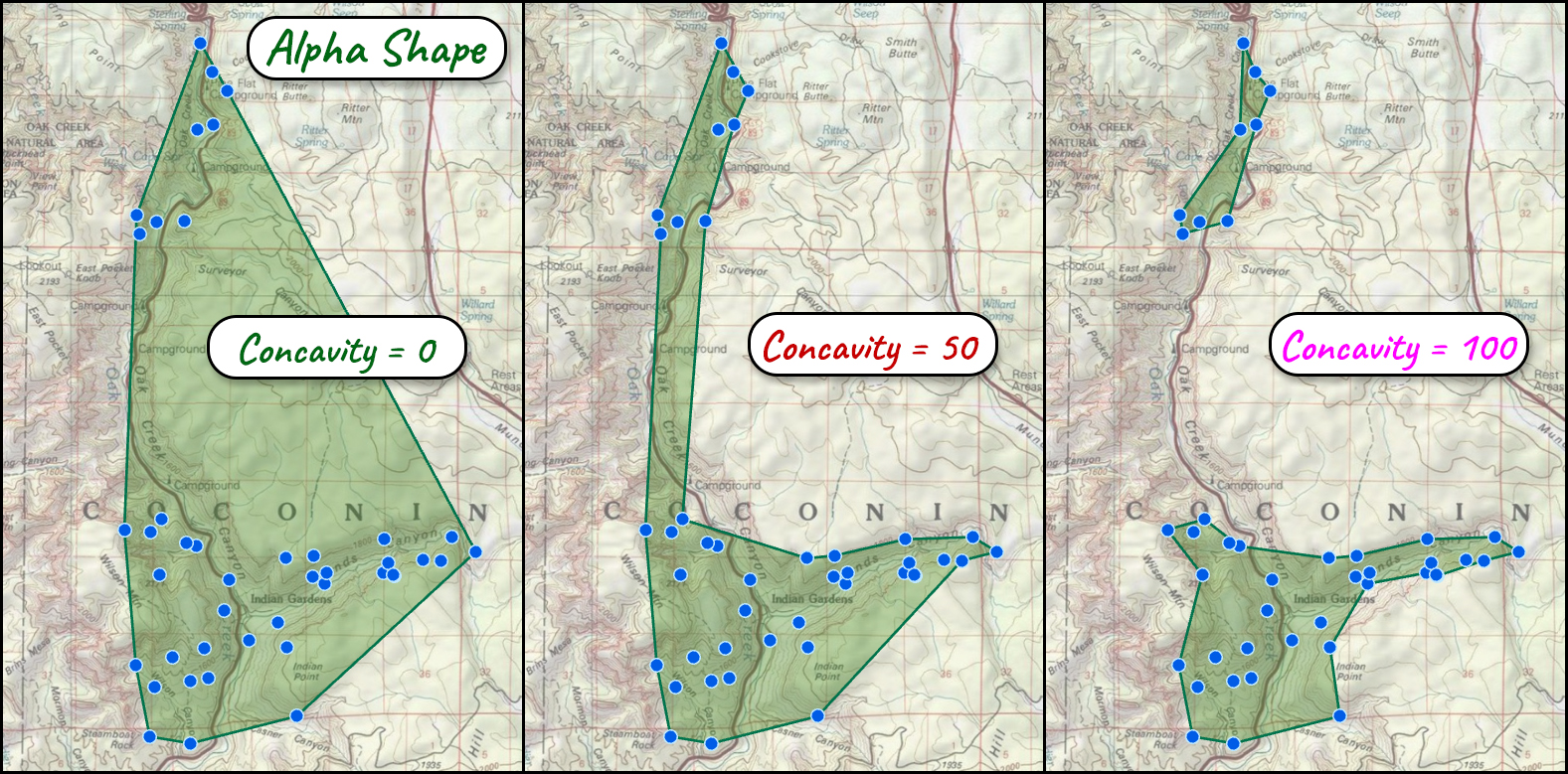
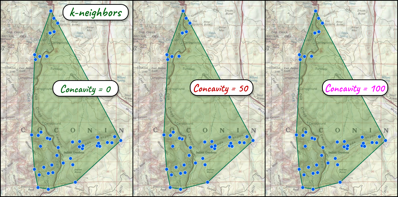
Why does the k-neighbours dial do so little here? The walk builds the boundary by stepping among each point's k nearest neighbours — and with two separated clusters, a walk with small k gets trapped circling one cluster: every one of its nearest neighbours is in the same cluster, so it closes a loop around those points and leaves the other individual's locations outside, which is not allowed. The walk cannot succeed until k is large enough that points across the gap count among the nearest neighbours — on this dataset, k = 30 of 43 points — and by then the boundary is nearly convex. The tool detects this: when a cloud's smallest workable k is above 3, it stretches the Concavity dial across the k range that actually exists and reports so in the run messages. But no setting can conjure concavity the method cannot deliver — a single k-neighbours walk around two separated clusters is nearly convex by nature. Contrast the k-neighbours panel of the three-methods figure above, where the locations span the canyon without a gap: there the walk carves a genuinely concave hull. For clustered data, reach for the alpha shape with parts allowed (one honest polygon per cluster), the chi shape (one polygon with a thin waist), or better yet a case field that puts each individual in its own group.

One hull per group

An optional case field builds one hull per field value — per animal, per survey period, per cluster ID. Each output hull carries its group value, its point count, the parameter actually used, its part and hole counts, and geodesic area and perimeter, so a season of telemetry becomes one row of honest footprint per animal in a single run.

MCP, LoCoH, Kernel Density — which home-range tool?

For home ranges and territories this tool sits in a family of choices. The classic minimum convex polygon is this tool at Concavity 0 (or Esri's Minimum Bounding Geometry): the conservative, capture-everything estimate, at the price of the plateau problem shown above. Two other tool families in this toolbox capture the shape of a point cloud, each answering a different research question. The Local Convex Hull (LoCoH) family unions many small local hulls, which not only follows the outline but also identifies areas of higher point density (utilization isopleths) — the standard approach for home-range estimation. The Enhanced Kernel Density tools give a heat-map version of the points' shape — a continuous density surface rather than a hard boundary — with contour and proportion companions for drawing density isopleths. If the question is “where do these points spend their weight” rather than “what outline do they occupy,” reach for LoCoH or Kernel Density; this tool is the better fit for a single clean footprint polygon.

Equivalents elsewhere

These are the same methods behind PostGIS's ST_ConcaveHull and SFCGAL ST_AlphaShape / ST_OptimalAlphaShape, CGAL's Alpha_shape_2, and the QGIS concave-hull processing algorithms (both its k-nearest-neighbours and alpha-shape variants) — so results can be matched across software. Esri's closest analog, Aggregate Points, requires an Advanced license; this tool runs at every license level.

What you get

One polygon feature class of hulls: the case-field value (when a case field is used), Method, NPoints, the parameter actually used (Param_m in meters for the alpha radius or chi edge length, or K_used for the k-NN hull), Parts and Holes counts, and geodesic Area_m2 and Perim_m. Measures that do not apply are null (−999 in shapefiles, which cannot store nulls).

Geometry notes

Layer selections are honored; duplicate points are dropped before analysis; groups with fewer than 3 distinct points are skipped with a warning. Geographic (latitude–longitude) points are solved in per-group azimuthal-equidistant working projections, and every area and perimeter is geodesic.

A tour of the dialog

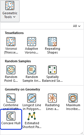
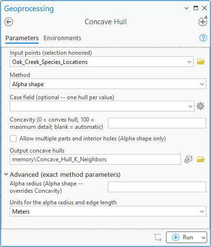
A basic run needs only the points, a method, and an output name — Concavity can stay blank for the automatic setting. The case field and the parts-and-holes checkbox (alpha only) cover grouping and cluster splitting, and the Advanced section holds the exact parameter for whichever method is chosen — the alpha radius below, since the method here is the alpha shape.

The Geometric Tools gallery open on the ribbon, with the Concave Hull button, in the Geometry on Geometry row, outlined in blue — Where to find it: **Concave Hull** is in the *Geometry on Geometry* row of the *Geometric Tools* gallery, in the Geometric Tools group of the *Wildlife and Forestry* tab.

The Concave Hull geoprocessing pane with the Oak Creek species locations as input, Alpha shape as the method, Concavity left blank for automatic, the parts checkbox unchecked, and the Advanced section expanded to show the alpha radius and its units dropdown — The dialog filled for an automatic alpha-shape run: points, method, output — Concavity left blank. The expanded Advanced section offers the exact alpha radius for when you know precisely what you want.

ModelBuilder

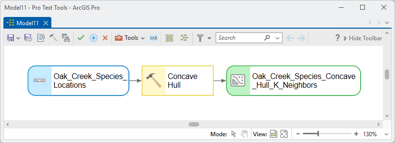
The hull feature class chains onward directly — as the clip or study-area polygon for later steps, the footprint whose Area_m2 feeds a report, or the per-animal outlines a model iterates over. Feeding a point layer in and reading the hull out is the whole pattern.

Parameters

Label	Explanation	Data type
Input pointsRequired · in_features	The point cloud to outline — telemetry fixes, plot locations, occurrence records. A layer selection is honored; duplicate points are dropped automatically.	Feature Layer
MethodRequired · method	Chi shape (characteristic shape), Alpha shape, or k-nearest-neighbours hull — see the three lineages above.	String
Case fieldOptional · case_field	Build one hull per value of this field — per animal, per survey period, per cluster.	Field
ConcavityOptional · concavity	0 = the convex hull, 100 = each method's maximum detail, blank = the method's moderate automatic setting. The Advanced exact parameters override it.	Double
Allow multiple parts and interior holesOptional · allow_parts	Alpha shape only: let the hull split into disjoint polygons and keep interior holes. Unchecked, the tool picks the smallest alpha keeping one piece.	Boolean
Output concave hullsRequired · out_features	The hull polygons: case value, Method, NPoints, Param_m or K_used, Parts, Holes, geodesic Area_m2 and Perim_m.	Feature Class
Alpha radiusOptional · alpha_radius	Advanced: the exact eraser-disk radius, in the units below; smaller hugs tighter (and may drop outlying points). Overrides Concavity for the Alpha method.	Double
Edge length thresholdOptional · chi_length	Advanced: the exact chi edge-length threshold, in the units below — boundary edges longer than this are carved away. Overrides Concavity for the Chi method.	Double
Number of neighbours kOptional · k_neighbors	Advanced: the exact starting k (at least 3); the tool settles on the smallest workable k at or above it and reports the k used. Overrides Concavity for the k-NN method.	Long
Units for the radius and edge lengthOptional · linear_units	Meters, Kilometers, Feet or Miles. Output measure fields are always meters.	String

Python

One automatic chi-shape hull per animal, then an alpha-shape run allowing separate parts and holes:

import arcpy
arcpy.ImportToolbox(r"C:\path\to\JennessEnterprisesTools.pyt")  # your install path
# method: "Chi shape (characteristic shape)" / "Alpha shape" /
#         "k-nearest-neighbours hull"
arcpy.jenness.ConcaveHull(
    in_features=r"D:\data\telemetry.gdb\fixes",
    method="Chi shape (characteristic shape)",
    case_field="Animal_ID",
    out_features=r"D:\data\telemetry.gdb\fix_outlines")
arcpy.jenness.ConcaveHull(
    in_features=r"D:\data\telemetry.gdb\fixes",
    method="Alpha shape",
    allow_parts=True,
    out_features=r"D:\data\telemetry.gdb\fix_alpha")

Recommended citation

Jenness, J. 2026. Concave Hull. Wildlife and Forestry Tools add-in for ArcGIS Pro, v. 1.98 (September 2026). Jenness Enterprises. Available at: https://github.com/JeffJenness/Wildlife_Tools.

Credits and references

By Jeff Jenness, Jenness Enterprises (www.jennessent.com), implementing the three classic concave-hull methods from their original papers.

Duckham, M., L. Kulik, M. Worboys, and A. Galton. 2008. Efficient generation of simple polygons for characterizing the shape of a set of points in the plane. Pattern Recognition 41:3224–3236. doi.org/10.1016/j.patcog.2008.03.023
Edelsbrunner, H., D. G. Kirkpatrick, and R. Seidel. 1983. On the shape of a set of points in the plane. IEEE Transactions on Information Theory 29:551–559. doi.org/10.1109/TIT.1983.1056714
Moreira, A., and M. Y. Santos. 2007. Concave hull: a k-nearest neighbours approach for the computation of the region occupied by a set of points. Pages 61–68 in Proceedings of the 2nd International Conference on Computer Graphics Theory and Applications (GRAPP 2007). doi.org/10.5220/0002080800610068

Licensing information

Works at every ArcGIS Pro license level (Basic, Standard, Advanced). No extension licenses are required — and Esri's closest analog, Aggregate Points, is itself an Advanced-license tool.

Voronoi (Thiessen) Polygons — the dual of the Delaunay triangulation the chi and alpha shapes are carved from.
Maximum Inscribed Geometry — the complementary question: not the outline around a cloud of points, but the largest shapes inside a polygon.
The LoCoH tools (Standard, Adaptive, Fixed Sphere) — local-hull home ranges with utilization isopleths.
The Kernel Density tools (Kernel Density Enhanced, KD to Proportion Surface, KD Probability Contours) — the heat-map version of a point cloud's shape.