

Centerline and Width
Summary
Collapses polygons — rivers, canals, corridors, valley bottoms — to their centerlines, carrying the local polygon width along every result. Output either the main centerline (the longest path through the polygon's medial axis) or the full branched skeleton with tributary branches, short boundary-noise spurs pruned. Every line carries minimum, mean, and maximum width in meters; optional station points carry the exact width at evenly spaced stations (the width profile), and optional segments carry width statistics per piece for graduated-color width maps. Interior holes are handled natively — the skeleton simply routes around islands — and any attribute fields transfer from the source polygons.
This is a license-free replacement for Esri's Polygon To Centerline, which requires Standard or Advanced plus the Production Mapping extension — and it computes widths, which Esri's tool does not attempt (see the comparison below).
From a ribbon of polygon to a line you can measure
Often the features we care most about arrive as long, thin polygons: a river digitized bank to bank, a wildlife corridor from a habitat model, a canyon bottom, a riparian strip. Two questions come up constantly with such shapes. Where is the middle? — because a centerline is what you measure distances along, chart conditions against, and label maps with. And how wide is it? — because width often drives ecological conditions: the narrows of a corridor could be bottlenecks to movement, the width of a river affects current speed and vegetation types, the width of a canyon or valley affects microclimate and habitat variability. This tool answers both questions in one pass, because the construction it uses cannot find the middle without also learning the width at every step.
How it works: the medial axis
Imagine standing inside the polygon and asking, at every point, “how far is the nearest bank?” That question always has a single answer — one shortest distance — but at special points the nearest bank itself is not unique: the same shortest distance is reached at two or more different places on the boundary. The medial axis — the polygon's skeleton — is the set of those points. Down the middle of a river channel, the nearest point on the left bank and the nearest point on the right bank are equally close — that is the centerline. The tool finds it by sampling the boundary densely, building the Voronoi diagram of those samples, and keeping the Voronoi vertices and edges that lie inside the polygon — the same construction our Bottleneck Analysis tool uses to find the pinch points in a corridor. And here is the free lunch: every skeleton point already knows its distance to the boundary — its clearance, which is exactly half the local polygon width. The centerline and the width are one object.
The main centerline is the longest path through that skeleton — the natural source-to-mouth line of a river polygon. One subtlety earned its place through real testing: where channels split and rejoin around an island, the longest path's ends are found by length, but the route between them weighs each step by its length divided by the local width — so the line follows the wider channel around an island rather than blindly the shorter one, matching what Bottleneck Analysis would choose and what a paddler would call the main channel.
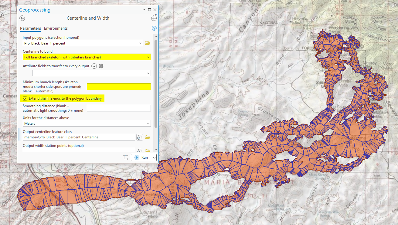
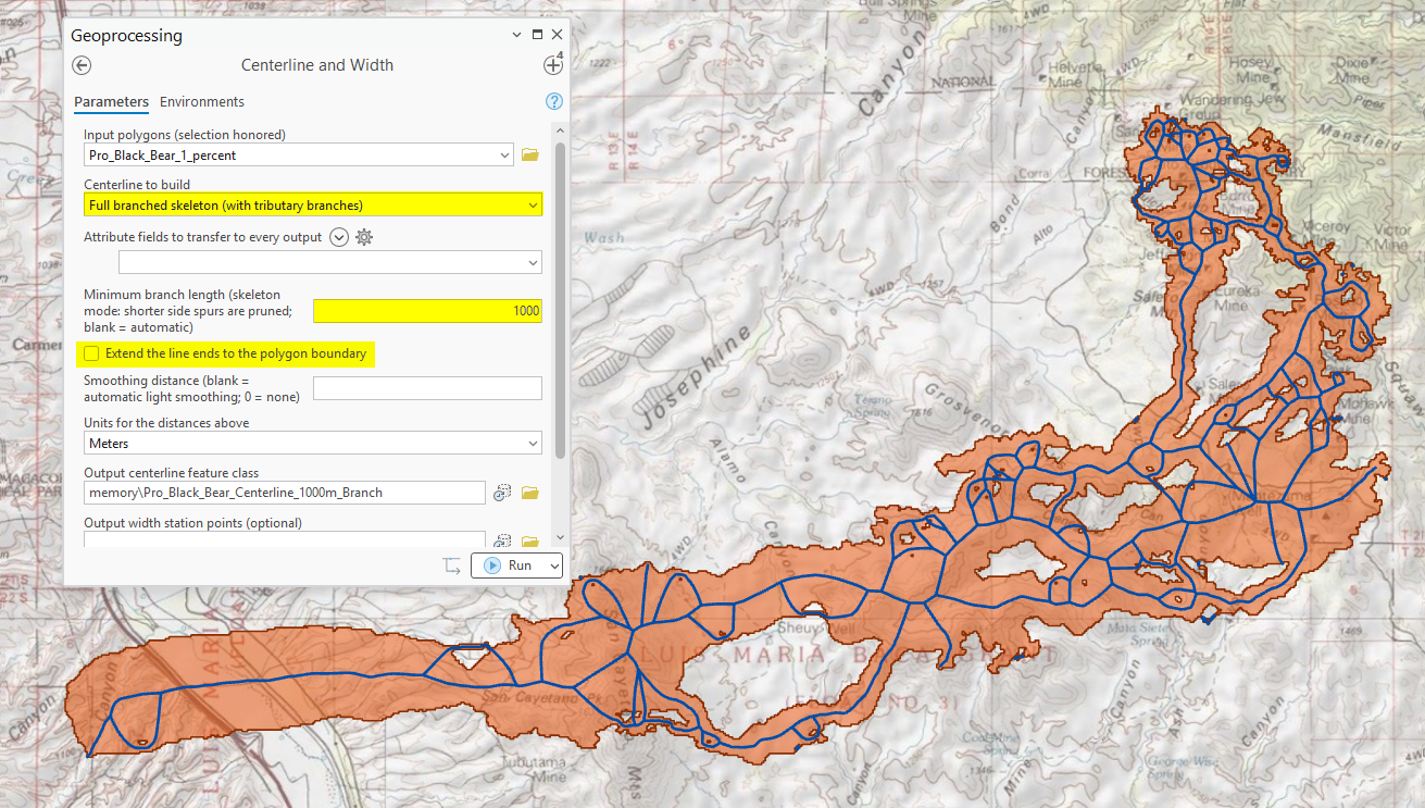
The two corridor figures in the next section show what the full skeleton actually looks like on real ground — and how the pruning control tames it.
Main centerline, or the full skeleton
Main centerline only gives one line per polygon (per part, for multipart inputs) — the spine.
Full branched skeleton keeps the tributaries: every branch becomes its own feature, split at junctions, and the IsTrunk field flags the pieces lying on the main centerline — so the main stem is one selection away from the full network. Side spurs shorter than the minimum branch length are pruned as boundary noise (branches on the main centerline are never pruned).
Choosing that minimum branch length is easiest by picture. Picture a river polygon about 100 m wide. Every irregularity in the bank — a cove, a backwater pocket, the stub of a side channel — sprouts its own short skeleton branch, roughly as long as the feature it reaches into. Left blank, only sampling-scale whiskers vanish, so all those coves keep their branches: the fullest skeleton. At 100 m — about the river's width — branches into mere bank features disappear, and what survives are genuine side channels and tributary arms longer than the river is wide: usually the natural choice. At 1,000 m, only major arms at least a kilometer long remain, collapsing a braided reach to its main stem and principal branches. In short: set it to the smallest side feature you would want to see as its own line. One practical note about polygons converted from rasters, such as corridors traced from a habitat model: their boundaries stair-step along the raster cell edges, and every square notch in that stair-stepping is a genuine boundary feature, not sampling noise — so the automatic pruning, which removes only sampling-scale whiskers, leaves thousands of short spurs, one reaching into each notch (the first corridor figure below shows the result). Setting the minimum branch length to roughly the corridor's width removes these cell-scale spurs and keeps only the branches that represent real arms of the corridor.
Widths everywhere
Every centerline carries MinW_m, MeanW_m, and MaxW_m plus its geodesic Length_m — all in meters, whatever units the dialog's distances use. Two optional outputs turn that summary into a profile:
- Station points — evenly spaced stations along every line, each with Station_m (distance along the line) and Width_m (the exact polygon width there). This is the width profile, ready to chart Width against Station or to join to field data. Leave the spacing blank and the tool places about 100 stations along the main centerline, then applies that same absolute spacing to every branch — a half-length branch gets ~50 stations, a stub gets its two endpoints — so station density stays uniform across the skeleton instead of piling 100 points onto every little spur.
- Segments — the centerline diced at those same stations, each piece carrying its own width statistics. Symbolize the segments with graduated colors and the river paints its own narrows.
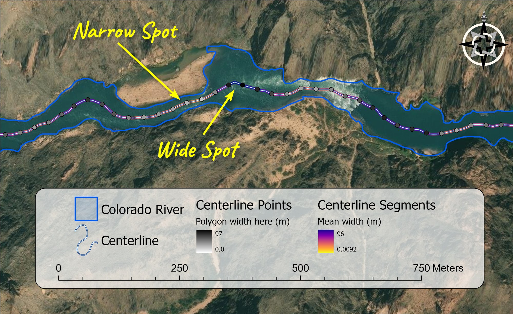
The Colorado River figure at the top of this page shows all three outputs working together: the station points shaded by Width_m are the width profile drawn directly on the map, and the graduated-color segments turn the same information into a reach-by-reach picture of the river's narrows and broads.
Ends, smoothing, and detail
A medial axis stops short of a polygon's end caps — the skeleton of a river dies out before the mouth. With Extend the line ends on (the default), each free tip is carried out to the boundary so centerlines reach their mouths; the near-zero widths on those short extension stubs are excluded from the line's width statistics, so a river's MinW_m reflects its real narrows, not the taper of its end cap. Smoothing relaxes the raw skeleton's jaggedness with a moving average — without ever letting the line leave the polygon (blank = automatic light smoothing; 0 = the raw skeleton). The Advanced Detail distance is the boundary sampling spacing behind the whole construction: smaller values resolve finer necks and tighter bends at more computing cost. If a run warns that the skeleton split into pieces at thin pinch points, lower it.
Holes, multipart polygons, and geographic data
Interior holes need no preprocessing: the skeleton routes around islands, and where a skeleton forms a ring around a hole it is written as a closed line. Multipart polygons yield one centerline per part, told apart by the Part field; every polygon in the input is processed, and a layer's selection is honored. True-curve boundaries (geodatabase circles and arcs) are densified automatically. Geographic (latitude–longitude) inputs are processed in a feature-centered equidistant projection, so all widths and lengths are honest meters.
Attribute transfer
Pick any of the source polygon's fields and every output feature — line, station point, and segment — carries them, alongside an automatic Src_FID (the source polygon's Object ID) and a Line_ID shared by a line and its points and segments, so the three outputs join to each other trivially. Fields whose names are reserved on the output (Shape_Length, Shape_Area…) or that collide with the tool's own fields still transfer — their source values arrive under a Src_ prefix, so Src_Shape_Area holds the source polygon's area, not anything about the line. Names are truncated and uniquified for shapefiles' 10-character attribute field name limit.
Relation to Esri's Polygon To Centerline
Esri's Polygon To Centerline (Topographic Production toolbox) requires a Standard or Advanced license plus the Production Mapping extension; this tool runs at every license level. Beyond licensing, the differences are substantive:
- Width — Esri's tool computes no widths at all; here every line, station, and segment carries them.
- Attributes — Esri's tool transfers nothing beyond an FID link; here any fields transfer.
- Holes — Esri's documentation directs users to remove interior holes with Eliminate Polygon Part before running, which destroys real islands; this tool handles holes natively and routes around them.
- Formats — Esri's tool supports neither shapefile output nor true-curve input; this tool supports both.
- Not replicated — Esri's Connecting Features parameter (snapping centerlines into an existing hydro network with flow direction) is the one capability this tool does not attempt.
A tour of the dialog
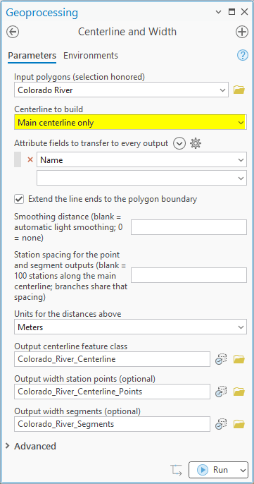
A basic run needs only the polygons, the centerline mode, and an output name; everything else has a sensible blank-equals- automatic default. The four distance entries (minimum branch length, smoothing, station spacing, Detail) share one units dropdown — and note that output width and length fields are always meters regardless.
ModelBuilder
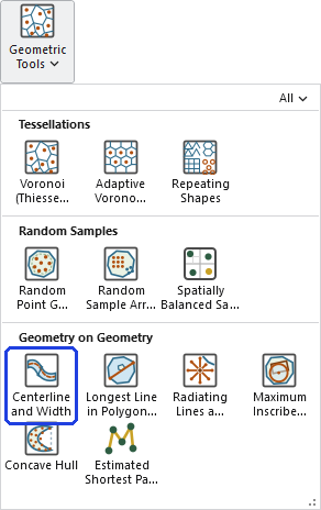
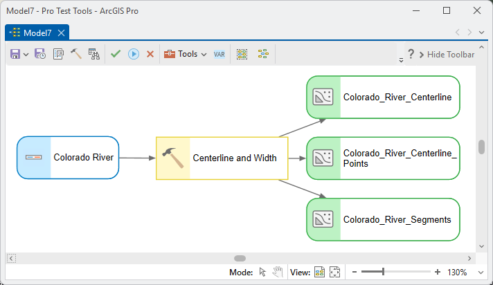
The tool hands a model up to three feature classes — centerlines, station points, and segments — each carrying Line_ID for joins, so a model can chain the stations straight into charting or the segments into symbology-ready layers.
Parameters
| Label | Explanation | Data type |
|---|---|---|
| Input polygonsRequired · in_features | The polygons to collapse to centerlines. Every polygon is processed; a layer selection is honored; holes are fine. | Feature Layer |
| Centerline to buildRequired · mode | Main centerline only (the skeleton's longest path), or the full branched skeleton with IsTrunk flagging the main line's pieces. | String |
| Attribute fields to transferOptional · transfer_fields | Any source fields, copied onto every output feature; reserved/conflicting names arrive under a Src_ prefix. Src_FID always carries the source Object ID. | Field (multiple) |
| Minimum branch lengthOptional · min_branch | Skeleton mode: side spurs shorter than this are pruned. Blank = automatic (whiskers only); about one polygon-width is usually the natural choice. Trunk pieces are never pruned. | Double |
| Extend the line endsOptional · extend_ends | Carries each free tip out to the polygon boundary so centerlines reach their mouths (default on); extension-stub widths are excluded from the statistics. | Boolean |
| Smoothing distanceOptional · smoothing | Moving-average smoothing that never lets the line leave the polygon. Blank = automatic light smoothing; 0 = none. | Double |
| Station spacingOptional · station_spacing | Distance between width stations for the point and segment outputs. Blank = the main centerline's length / 100, applied as the same spacing to its branches. | Double |
| Units for the distances aboveOptional · linear_units | Meters, Kilometers, Feet or Miles — for the four distance entries. Output width/length fields are always meters. | String |
| Output centerline feature classRequired · out_lines | Line_ID, Src_FID, Part, IsTrunk, geodesic Length_m, MinW_m / MeanW_m / MaxW_m, plus transferred fields. | Feature Class |
| Output width station pointsOptional · out_points | Evenly spaced stations with Station_m and Width_m — the width profile. | Feature Class |
| Output width segmentsOptional · out_segments | The centerline diced at the stations, each piece with its own width statistics. | Feature Class |
| Detail: boundary sampling distanceOptional · boundary_step | Advanced: the sampling spacing behind the skeleton (blank = automatic, ~1/2000 of each polygon's extent diagonal). Lower it if thin necks disconnect the skeleton. | Double |
Python
A river polygon collapsed to its main centerline with a width profile every 100 m, carrying the river's name:
import arcpy
arcpy.ImportToolbox(r"C:\path\to\JennessEnterprisesTools.pyt")  # your install path
# mode options (matching is by prefix):
#   "Main centerline only"
#   "Full branched skeleton (with tributary branches)"
# linear_units: "Meters" / "Kilometers" / "Feet" / "Miles"
#   (applies to min_branch, smoothing, station_spacing, boundary_step;
#    output width/length FIELDS are always meters)
arcpy.jenness.CenterlineAndWidth(
    in_features=r"D:\data\hydro.gdb\river_polys",
    mode="Main centerline only",
    transfer_fields="GNIS_Name",
    extend_ends=True,
    station_spacing=100.0,
    linear_units="Meters",
    out_lines=r"D:\data\hydro.gdb\river_centerlines",
    out_points=r"D:\data\hydro.gdb\river_width_stations",
    out_segments=r"D:\data\hydro.gdb\river_width_segments")
Recommended citation
Credits
By Jeff Jenness, Jenness Enterprises (www.jennessent.com). The centerline is the polygon's medial axis, extracted from the Voronoi diagram of densely sampled boundary points — the same engine that powers this suite's Bottleneck Analysis tool, where the identical skeleton-with-clearance construction finds a corridor's pinch points instead of the longest line down its middle.
Licensing information
Works at every ArcGIS Pro license level (Basic, Standard, Advanced). No extension licenses are required — unlike Esri's Polygon To Centerline, which needs Standard or Advanced plus the Production Mapping extension.
Related tools and pages
- Bottleneck Analysis — the same medial-axis engine pointed at a different question: where a corridor pinches, and how wide its bottlenecks are.
- Voronoi (Thiessen) Polygons — the construction underneath the medial axis, as a tool in its own right.
- Estimated Shortest Path through Points — turn the width stations you plan to visit into an efficient field route.