Maximum Inscribed Geometry

Geometric Tools · geoprocessing tool · by Jeff Jenness

Works at every ArcGIS Pro license level

Summary

Finds the largest circle, rectangle, convex polygon (MCP) or ellipse — or all four — that fits entirely inside each polygon, with interior holes acting as barriers. This is the deliberate dual of Esri's Minimum Bounding Geometry, which fits shapes around features; no Esri tool at any license level fits them inside. The circle is exact; the rectangle searches every orientation (or one you fix); the convex polygon is the classic potato peeling problem of computational geometry; the ellipse is always genuinely inside. Every shape carries its geodesic area and dimensions.

The biggest thing that fits

A surprising number of field questions reduce to “what is the biggest X that fits in here?” The widest circular habitat core a patch can hold — the largest buffer you could draw without touching an edge — is a core-area measure with the edge effects already subtracted. The largest rectangle inside a corridor is the biggest study plot or treatment unit the ground can accommodate, and a fixed azimuth turns it into the biggest plot that runs north–south. The largest convex region among barriers is the roomiest open ground an animal could cross without cover. And the largest inscribed ellipse summarizes a patch's usable interior in the same language as home-range ellipses. Interior holes — buildings, water, rock outcrops, excluded habitat — act as barriers every shape must avoid, exactly as islands block the Longest Line in Polygon (Fetch) tool. Computational geometers call these the “stick” and “potato” problems — the longest segment and the fattest convex body in a polygon — and the two tools form that pair deliberately.

A modeled black bear movement corridor in southern Arizona, an irregular orange polygon full of interior holes, with its four inscribed shapes drawn: a yellow circle in the broad northeastern lobe, and a magenta rectangle, blue ellipse, and green convex polygon overlapping each other in the long straight southwestern arm near Tubac — The whole tool in one figure: an “All four” run on a modeled black bear movement corridor in southern Arizona. Notice that the four winners did not agree on a location — the largest circle (yellow) found the corridor's widest ground in the northeastern lobe, while the rectangle (magenta), ellipse (blue), and convex polygon (green) all settled into the long, straight southwestern arm. The white gaps inside the corridor are holes (presumably containing unsuitable habitat black bears would avoid): excluded ground every shape must avoid.

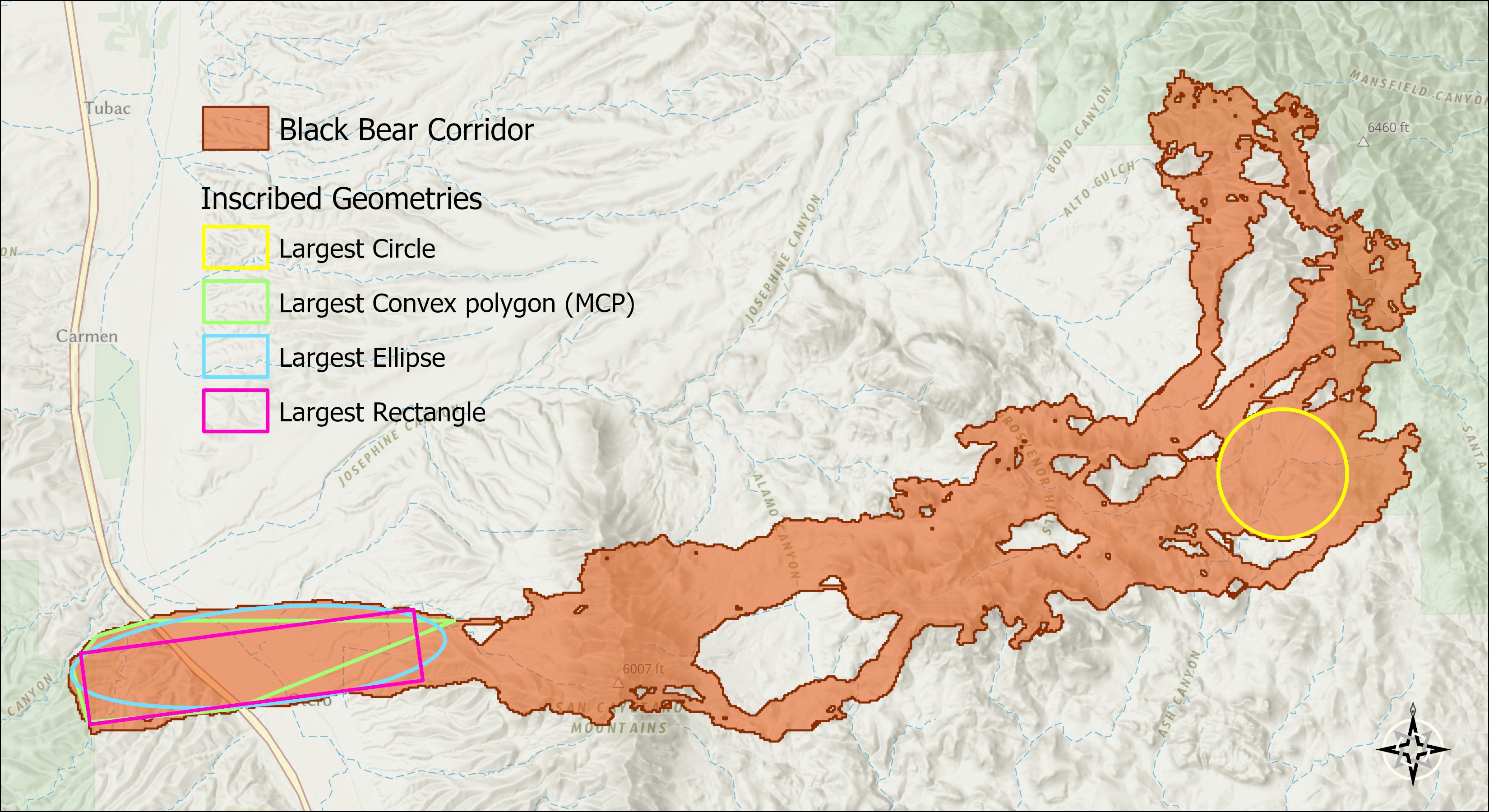
The dual of Minimum Bounding Geometry

Esri's Minimum Bounding Geometry answers “what is the smallest circle / rectangle / hull around this feature?” — useful, but a bounding shape says nothing about what the polygon can contain. A crescent and a disk of the same extent get similar bounding circles, while the crescent can hold only a small inscribed one: the inscribed shapes measure the polygon's usable interior, its compactness in a way perimeter ratios cannot, and the size of the largest disturbance-free zone it offers. This tool is the other half Esri never built.

The four shapes, and how each is found

Circle — exact. The center of the largest inscribed circle always sits on the polygon's medial axis — the same skeleton-of-equidistant-points that powers our Centerline and Width tool — because a circle that touches only one stretch of boundary can always slide away from it and grow. The tool finds the best skeleton vertex and then polishes the center against the true boundary. The result is the polygon's “widest spot”: the largest circular buffer it can contain, reported with Radius_m.

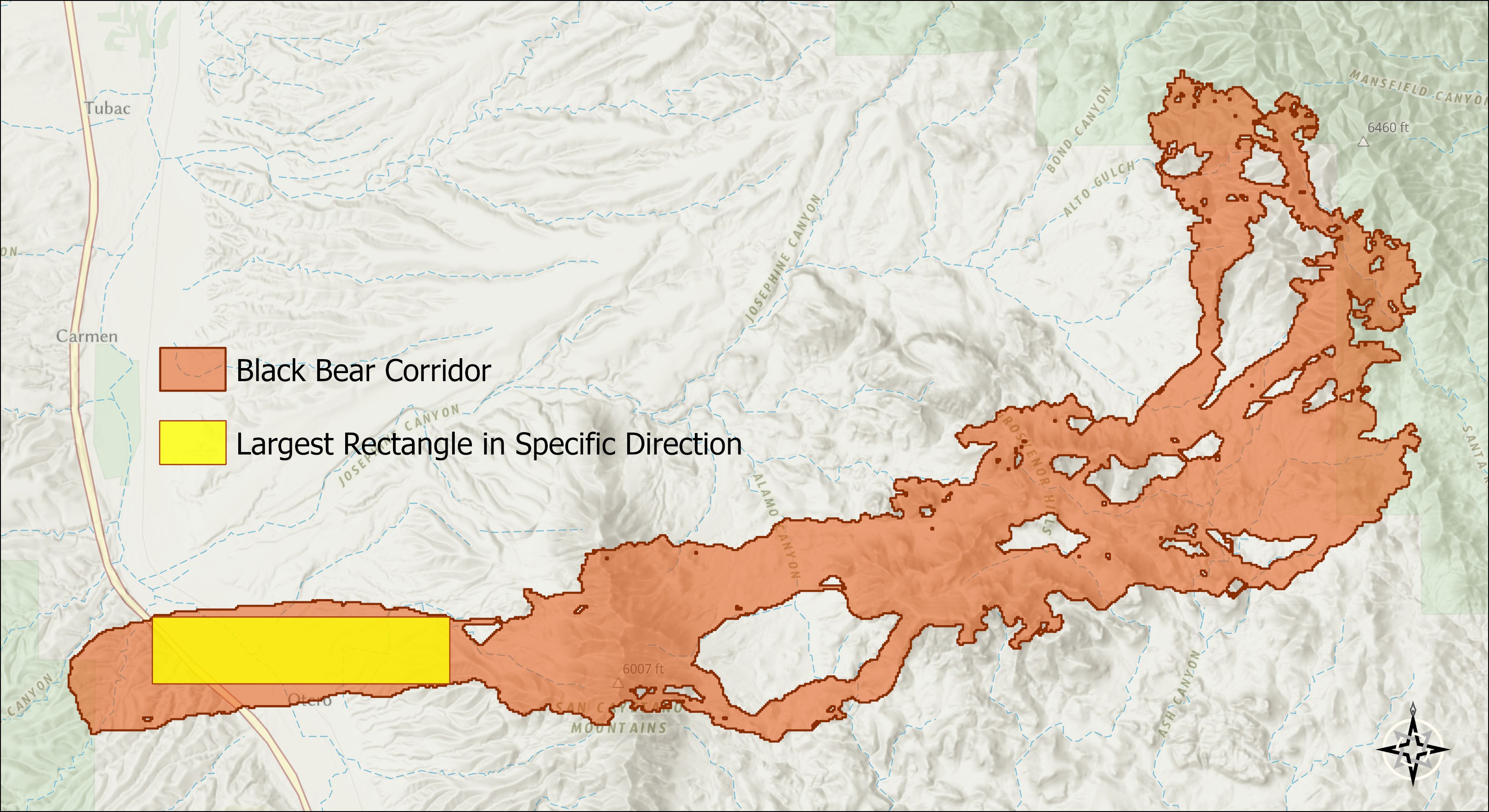
Rectangle — every orientation, then the true boundary. The tool sweeps the full range of orientations, solves each one exactly on a fine grid, refines the most promising angles on finer grids, and finally pushes all four sides outward against the true boundary until each one touches. Give a fixed azimuth (Advanced) and the sweep is skipped — the rectangle runs at your orientation, for survey plots that must align with a bearing or a management grid. Reported with Length_m, Width_m, and Azimuth.

The fixed azimuth matters because developers and planners often need the development itself to run in a particular direction — solar arrays oriented for sun exposure, an airstrip along the prevailing wind, crop rows or survey grids laid out on cardinal bearings, a building footprint square to an existing road. The free search answers “what is the largest rectangle at any orientation?”; the fixed azimuth answers the question those projects actually ask: “what is the largest rectangle at my orientation?”

The same black bear corridor polygon with a single yellow rectangle inscribed in the southwestern arm, held exactly east-west rather than tilted along the arm — The same corridor with the rectangle held to an east–west bearing. It is smaller than the free-search rectangle in the figure above, which was allowed to tilt with the arm — but it is exactly what a project laid out on cardinal bearings could actually use.

Convex polygon (MCP) — the potato-peeling problem. The largest convex region inside a polygon is a famous problem with a humbling pedigree: an exact solution on the continuous polygon exists (Chang and Yap 1986) but takes on the order of n⁷ time — for a thousand-vertex boundary, arithmetic in the ten-sextillion-operation range, hopeless in practice. Following the spirit of Aronov, van Kreveld, Löffler and Silveira's Peeling Meshed Potatoes (2011), this tool instead solves the problem exactly on a discretization — candidate points at the Detail spacing plus the polygon's own vertices — and then polishes the winning shape outward against the true boundary. The result is always truly convex and truly inside, and a finer Detail can only enlarge it. A convex input returns itself, exactly. Think of it as the largest region a Minimum Convex Polygon home range could occupy without touching any barrier.

Ellipse — a five-dimensional shortcut, then the true boundary. The ellipse search uses the elegant conic-linearization method of Hall-Holt, Katz, Kumar, Mitchell and Sityon (2006): every ellipse's equation is linear in five coefficients, so boundary sample points can be “lifted” into a five-dimensional space where candidate maximum ellipses become facets of a convex hull — a geometric trick that turns an unruly search into hull computation. The candidates, plus warm starts from the circle, the rectangle, and the convex polygon's inner ellipse, are then polished directly against the true boundary edges and shrunk-to-fit, so the reported ellipse is always genuinely inside. Reported with MajAxis_m, MinAxis_m, and Azimuth; for convex inputs the answer is exact.

Interior holes are barriers — a Coconino example

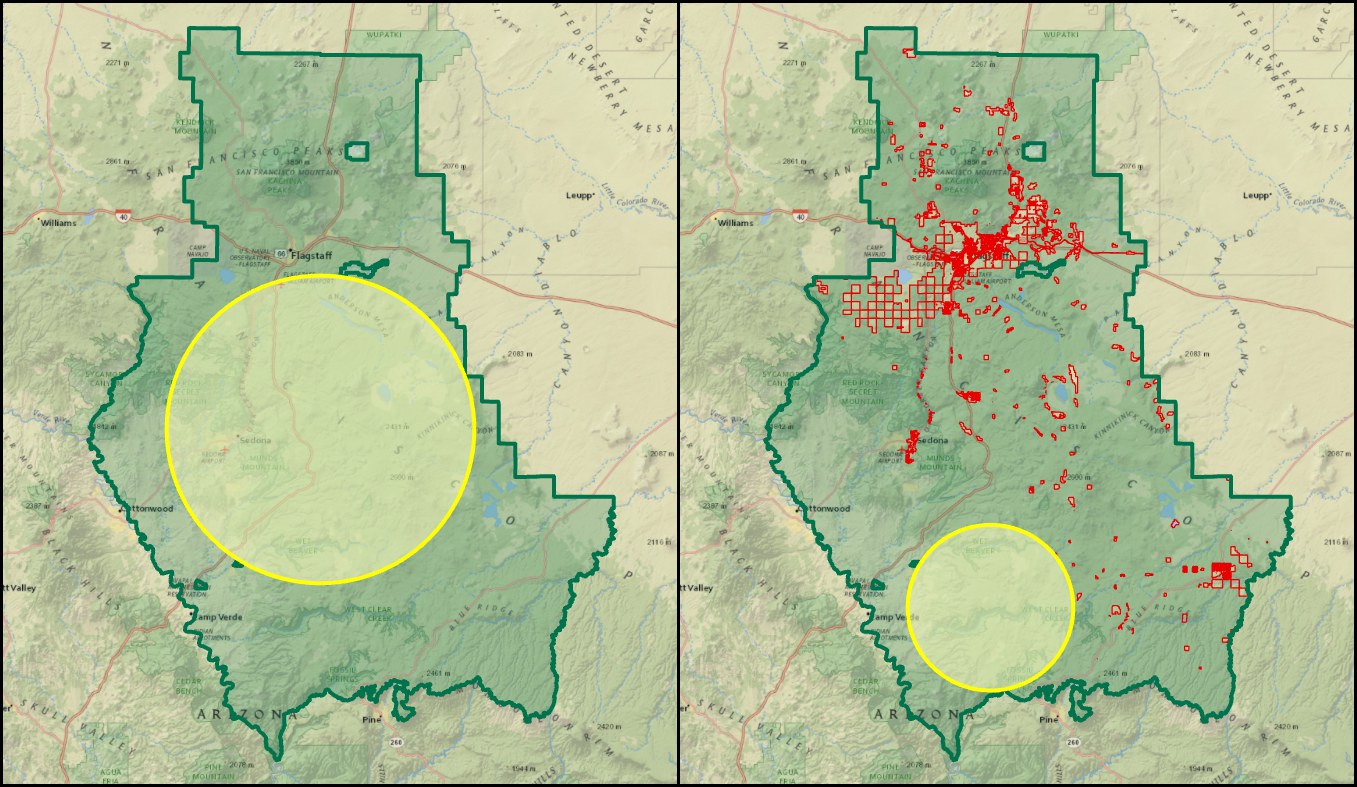
Suppose we want the largest contiguous circle of National Forest land in the Coconino National Forest of northern Arizona. It is tempting to run the tool on the forest boundary as published and take the answer on the left below — a generous circle sweeping from Sedona most of the way to Flagstaff. But that answer is naive. Like most western forests, the Coconino is riddled with private inholdings — the red parcels on the right — and the land inside the boundary is not all Forest land. Punch the inholdings out of the boundary polygon so they become interior holes, and the honest answer is the much smaller circle in the quieter country around West Clear Creek. Every shape treats holes this way: they are barriers the shape must stay clear of, never blemishes it may cover.

Two maps of the Coconino National Forest side by side. On the left, a large yellow inscribed circle spans the country between Sedona and Flagstaff. On the right, hundreds of small red private-inholding parcels are drawn inside the forest boundary and the inscribed circle is far smaller, relocated south to the West Clear Creek area — The largest circle of contiguous National Forest land, computed two ways. Left: the boundary as published, ignoring ownership. Right: with the private inholdings (red) punched out as holes, the largest circle that avoids them all is dramatically smaller and lives somewhere else entirely.

What you get

One polygon feature class. You can ask for any one of the four shapes individually, or for all four at once. A single-shape run yields one row per input feature; with “All four,” each input feature yields one row per shape, told apart by Shape_Kind. Every row carries the geodesic Area_m2, the center coordinates, and its own measures — Radius_m for the circle; Length_m, Width_m and Azimuth for the rectangle; MajAxis_m, MinAxis_m and Azimuth for the ellipse; NumVerts for the convex polygon — plus Src_FID, Part (which part of a multipart feature holds the winner), and any transferred attribute fields (reserved names arrive under a Src_ prefix). Measures that do not apply to a shape are null (−999 in shapefiles, which cannot store nulls).

Speed, Detail, and the simplify tolerance

The Advanced Detail distance sets the working resolution for all four shapes — the boundary sampling, the rectangle's grids, and the convex polygon's candidate points (blank picks about 1/150 of each feature's extent). Its practical effect differs by shape, and the difference is worth knowing: the convex polygon is the shape genuinely sensitive to it, because its vertices come from candidates spaced at this distance, so a finer Detail can find a genuinely larger polygon. The circle, rectangle, and ellipse are all refined against the true boundary afterward, so for them Detail mostly trades speed for search thoroughness rather than final precision.

The simplify tolerance pre-simplifies each boundary before any fitting, exactly as in the Fetch tool — and for the same reason: a raster-traced polygon carries a stair-step vertex at every cell corner, detail that describes the cell size rather than the shape. A tolerance near the cell size removes those vertices and speeds every stage, while the shapes can shift by roughly the tolerance. The progress bar names each polygon and stage as the tool works.

Geographic data

Layer selections are honored; multipart features report the best shape over their parts; true-curve boundaries are densified automatically. Geographic (latitude–longitude) polygons are solved in per-feature azimuthal-equidistant working projections, so radii, lengths, and areas are true geodesic meters at any latitude.

A tour of the dialog

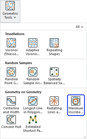
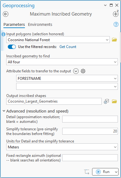
A basic run needs the polygons, a shape choice, and an output name. The Advanced section holds Detail, the simplify tolerance, their shared units dropdown, and the rectangle's fixed azimuth. Below, the pane is filled for the Coconino run: all four shapes, the FORESTNAME field carried to the output, and a 20 m simplify tolerance to thin the finely traced boundary before any fitting begins.

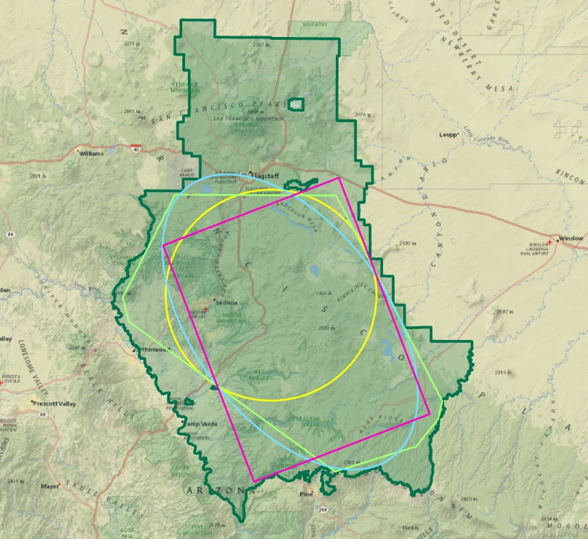
The Geometric Tools gallery open on the ribbon, with the Maximum Inscribed Geometry button, in the Geometry on Geometry row, outlined in blue — Where to find it: **Maximum Inscribed Geometry** is in the *Geometry on Geometry* row of the *Geometric Tools* gallery, in the Geometric Tools group of the *Wildlife and Forestry* tab.

The Maximum Inscribed Geometry geoprocessing pane with Coconino National Forest as the input, All four as the geometry, FORESTNAME as the transfer field, Coconino_Largest_Geometries as the output, and a 20 meter simplify tolerance set in the expanded Advanced section — The dialog filled for an “All four” run on the Coconino National Forest boundary.

…which produces this:

The Coconino National Forest boundary with all four inscribed shapes drawn together: a yellow circle, green convex polygon, blue ellipse, and magenta rectangle, all overlapping across the forest's broad central country between Sedona and Flagstaff — All four inscribed shapes for the Coconino boundary — circle (yellow), convex polygon (green), ellipse (blue), and rectangle (magenta). This run used the boundary as published; compare the inholdings-aware circle in the section above.

ModelBuilder

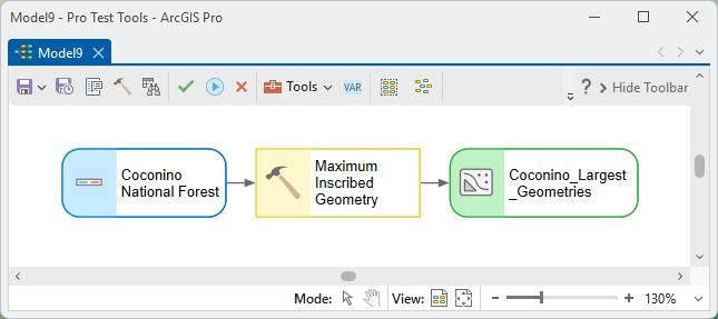
In a model, the cleanest way to hand a single shape to the next tool in the chain is to generate only that shape: set “Inscribed geometry to find” to the one you need, and the output holds exactly one row per input feature, ready to feed straight onward — the inscribed circles alone as habitat cores, say. If downstream tools want to work with several of the shapes from an “All four” run, Shape_Kind is the handle: a Select By Attributes pulls each kind into its own branch, or an iterator can walk the shapes one at a time.

Parameters

Label	Explanation	Data type
Input polygonsRequired · in_features	The polygons to fit shapes inside — habitat patches, forest gaps, lakes, corridors. Interior holes act as barriers. A layer selection is honored.	Feature Layer
Inscribed geometry to findRequired · geometry_type	Circle, Rectangle, Convex polygon (MCP), Ellipse, or All four (one row per shape, told apart by Shape_Kind).	String
Attribute fields to transferOptional · transfer_fields	Source fields copied onto every output shape; reserved names arrive under a Src_ prefix.	Field (multiple)
Output inscribed shapesRequired · out_features	Src_FID, Part, Shape_Kind, geodesic Area_m2, center coordinates, and each shape's own measures, plus transferred fields.	Feature Class
DetailOptional · detail	Advanced: the working resolution for all four shapes (blank = about 1/150 of each feature's extent). The convex polygon is the shape genuinely sensitive to it.	Double
Simplify toleranceOptional · simplify_tolerance	Advanced: pre-simplify each boundary before fitting, as in the Fetch tool; shapes can shift by roughly the tolerance. Blank = the exact boundary.	Double
Units for Detail and the toleranceOptional · linear_units	Meters, Kilometers, Feet or Miles. Output measure fields are always meters.	String
Fixed rectangle azimuthOptional · fixed_azimuth	Advanced, rectangle only: constrain the rectangle to one orientation (degrees clockwise from north); blank searches all orientations.	Double

Python

All four inscribed shapes for every habitat patch, with a simplify tolerance for raster-traced boundaries:

import arcpy
arcpy.ImportToolbox(r"C:\path\to\JennessEnterprisesTools.pyt")  # your install path
# geometry_type: "Circle" / "Rectangle" / "Convex polygon (MCP)" /
#                "Ellipse" / "All four"
# linear_units:  "Meters" / "Kilometers" / "Feet" / "Miles"
arcpy.jenness.MaximumInscribedGeometry(
    in_features=r"D:\data\habitat.gdb\patches",
    geometry_type="All four",
    transfer_fields="Patch_Name",
    out_features=r"D:\data\habitat.gdb\patches_inscribed",
    simplify_tolerance=30.0, linear_units="Meters")

Recommended citation

Jenness, J. 2026. Maximum Inscribed Geometry. Wildlife and Forestry Tools add-in for ArcGIS Pro, v. 1.98 (September 2026). Jenness Enterprises. Available at: https://github.com/JeffJenness/Wildlife_Tools.

Credits and references

By Jeff Jenness, Jenness Enterprises (www.jennessent.com). The convex-polygon method follows the discretize-then-solve approach of Aronov and colleagues' Peeling Meshed Potatoes; the ellipse method follows the conic linearization of Hall-Holt and colleagues' Finding Large Sticks and Potatoes in Polygons.

Aronov, B., M. van Kreveld, M. Löffler, and R. I. Silveira. 2011. Peeling meshed potatoes. Algorithmica 60:349–367. doi.org/10.1007/s00453-009-9346-8
Chang, J. S., and C. K. Yap. 1986. A polynomial solution for the potato-peeling problem. Discrete & Computational Geometry 1:155–182. doi.org/10.1007/BF02187692
Hall-Holt, O., M. J. Katz, P. Kumar, J. S. B. Mitchell, and A. Sityon. 2006. Finding large sticks and potatoes in polygons. Pages 474–483 in Proceedings of the 17th ACM-SIAM Symposium on Discrete Algorithms (SODA). ACM Digital Library · author's copy (PDF)

Licensing information

Works at every ArcGIS Pro license level (Basic, Standard, Advanced). No extension licenses are required — and Esri offers no inscribed-geometry tool at any license level; Minimum Bounding Geometry solves only the outside-fitting dual.

Longest Line in Polygon (Fetch) — the “stick” to this tool's “potatoes”: the longest straight line inside each polygon.
Centerline and Width — the medial axis behind the exact inscribed circle, as a tool of its own.
Voronoi (Thiessen) Polygons — the construction underneath the medial axis.
Bottleneck Analysis — the same medial-axis machinery pointed the other way: where this tool finds the biggest shapes a corridor can hold, that one finds the pinch points that constrain it.
Concave Hull — the complementary question: not the largest shapes inside a polygon, but the outline around a cloud of points.