

Adaptive Voronoi Polygons
Summary
Subdivides a boundary polygon into compact, nearly equal-area Voronoi cells arranged in a honeycomb-like pattern. Voronoi polygons are generated around seed points (the features of a point feature class, or a chosen number of random points placed inside the boundary), clipped to the boundary, and each point then moves to its clipped cell's centroid; the process repeats until the cells settle, the iteration limit is reached, or the time limit expires. Over the iterations the cell areas draw together — an ecologically defensible way to cut an analysis or management area into workable, near-circular pieces rather than narrow slices. Geographic data is tessellated exactly on the sphere.
Use it wherever an area needs to become units: survey blocks of comparable effort, management parcels of comparable size, or territory-like partitions grown outward from real sites. There is no standard Esri geoprocessing tool that performs this subdivision.
Usage
The method: Lloyd's algorithm and the centroidal Voronoi tessellation
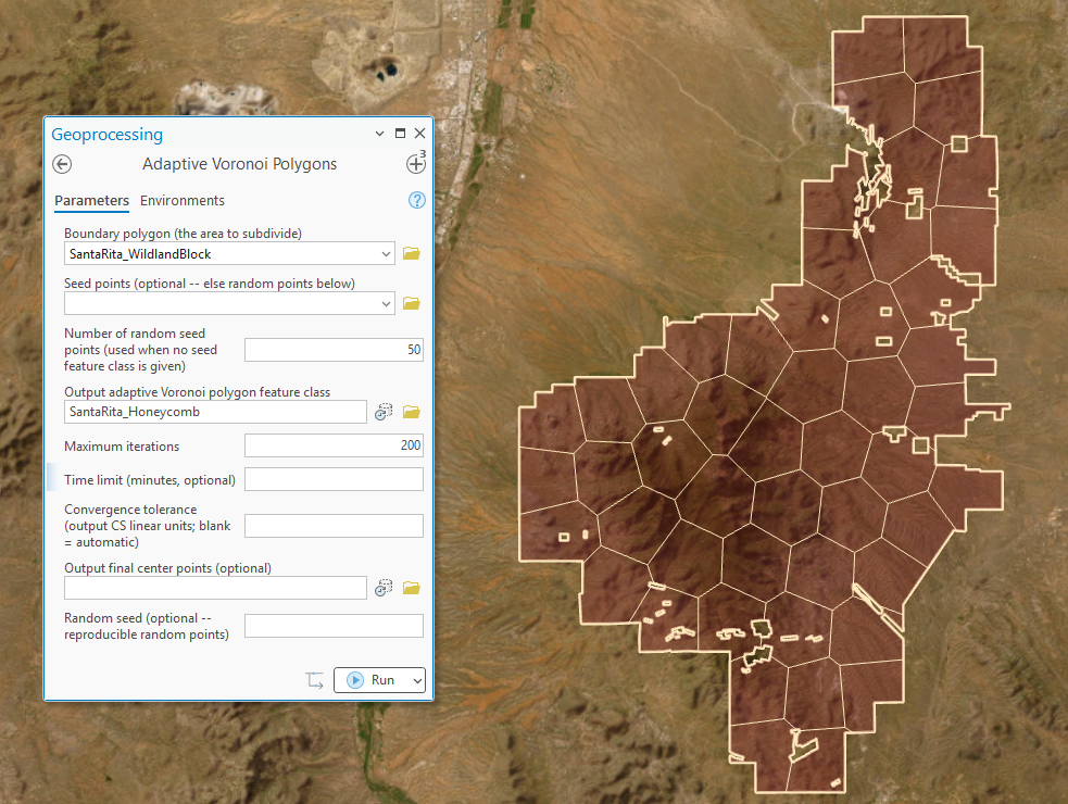
The method is Lloyd's algorithm (Lloyd 1982), and the pattern it settles into is a centroidal Voronoi tessellation (CVT): a Voronoi diagram whose every generating point coincides with its own cell's centroid (Du, Faber and Gunzburger 1999). Each iteration is simple — tessellate, clip to the boundary, move every point to its clipped cell's centroid — and repetition does the rest: crowded points spread apart, lonely points' cells shrink toward their neighbors', and the areas draw together. With uniform density the optimal cells approach congruent regular hexagons (Gersho's conjecture), which is why the finished result looks like a honeycomb of compact, nearly equal-area partitions molded to the boundary.
One detail worth being precise about, because the result depends on it: every centroid is the centroid of the clipped cell — the part inside the boundary — never of the full unclipped polygon. That is what molds the honeycomb to the boundary's shape instead of letting edge cells drift outward.
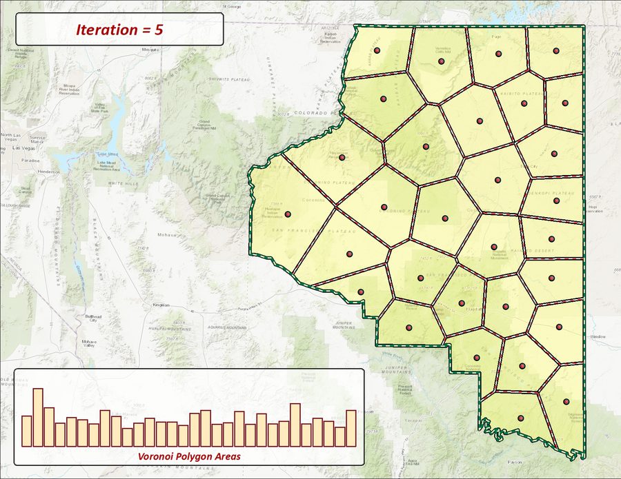
To see the process itself rather than just where it ends, a short video shows a set of points evolving into an adaptive Voronoi tessellation, iteration by iteration — the cells trading ground while the histogram of their areas pulls level:
Honeycombs in nature
Nature ran this algorithm long before we did. That territories should become hexagonal at high density in a uniform environment is an old prediction of theoretical ecology, but documenting it proved stubbornly difficult until Barlow (1974) photographed breeding male Tilapia mossambica in a Berkeley pool with a uniform sand bottom. Each jet-black male excavates a breeding pit by spitting sand away from the pit's center — in Barlow's words, “often toward rival males” — and where two territories meet, the reciprocal spitting piles up a sand parapet: a boundary built by equal-and-opposite antagonism, which is to say a physical perpendicular bisector. Isolated pits were always circular; wherever pits touched, the shared edges straightened; and when the density of breeding males rose from 46 pits to 73, the proportion of hexagonal territories nearly doubled while the pits' mean size held constant — the packing simply became more efficient, and the unoccupied scraps between territories vanished. Barlow could even read social standing in the geometry: a straight boundary meant the neighbors were equals, while a side bowed outward marked the slightly dominant male pushing his wall toward a subordinate.
The parallel with this tool runs deep, right down to the imperfections: Barlow found that pentagons remained the most frequent shape even at high density, and a centroidal tessellation confined by a real boundary likewise settles into a mixture of pentagons and hexagons rather than a perfect honeycomb. His Plate XIV photograph of the polygonal pit array — reproduced by Du, Faber and Gunzburger to open their survey's applications — is worth the trip to the original (doi.org/10.1016/0003-3472(74)90010-4), and he suspected the same geometry wherever territories are small enough for their occupants to tend every boundary at once, from cichlid breeding arenas to densely nesting colonial terns.
Stopping
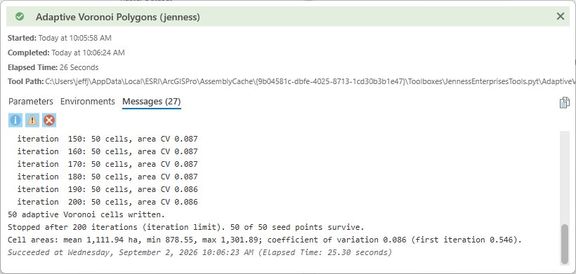
The run ends at whichever comes first of the iteration limit, the time limit, or convergence — no centroid moved farther than the tolerance between iterations (the default tolerance is 0.05% of the mean cell diameter). Lloyd's algorithm converges geometrically, so well-behaved runs usually stop on convergence long before a generous iteration limit. The messages report the cell count and the coefficient of variation (CV) of the cell areas as the run progresses, and the final area statistics. The CV is the standard deviation of the cell areas divided by their mean — a unitless measure of relative spread, so it reads the same in any area unit. A line like “area CV 0.086” says the cells' areas typically sit within about 9% of the mean; a fresh random tessellation starts near 0.5, and perfectly equal areas would be 0. Watch it fall as the areas equalize.
Seeds and survival
Seeds come from a point feature class (selection honored, multipoints exploded, each surviving cell carrying a Seed_FID back to its seed) or as random points placed uniformly inside the boundary — equal-area sampling on the sphere for geographic data, with the random seed making runs exactly reproducible. All points always participate: there is deliberately no “use only points inside the boundary” option on this tool. A point is lost only when its clipped cell disappears entirely outside the boundary, and the iteration continues with the survivors.
Relation to the Voronoi (Thiessen) Polygons tool
This tool runs the Voronoi (Thiessen) Polygons within Boundary tool's tessellation engines iteratively, with two deliberate differences. There is no only-points-inside option (see above). And geographic data uses the exact-sphere engine without the ellipsoidal refinement — the sub-0.5% spherical difference is irrelevant to where the iteration settles, and skipping it keeps every iteration fast.
Speed
Each iteration, only the cells actually touching the boundary edge are clipped with exact geometry; the interior cells — the bulk, and a growing share as the cell count grows — take a fast numerical path, and real output geometries are built once, at the end. A few hundred cells over a few hundred iterations completes in seconds; the time limit exists for very large runs. The Output Coordinate System environment is honored (defaulting to the boundary's coordinate system), and a seed feature class in a different coordinate system is projected automatically.
ModelBuilder
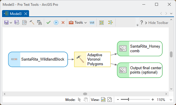
The tool offers two outputs to a model: the cell polygons (Cell_ID, Area_Ha, and Seed_FID for feature-class seeds) and the optional final center points — the honeycomb's generating points, with matching Cell_ID — ready for Random Point Generator sampling within cells or Select Random Records subsetting:
Parameters
| Label | Explanation | Data type |
|---|---|---|
| Boundary polygonRequired · boundary | The polygon to subdivide. Multiple polygons are unioned; holes are respected (cells never cover them); a map layer's selection is honored. | Feature Layer |
| Seed pointsOptional · in_points | Optional starting points. Each surviving cell carries a Seed_FID linking it back to its seed point. A selection is honored; multipoints are exploded. Leave blank to use random seed points instead. | Feature Layer |
| Number of random seed pointsOptional · n_random | How many cells to create when no seed feature class is given: this many random points are placed uniformly inside the boundary (equal-area sampling on the sphere for geographic data). | Long |
| Output adaptive Voronoi polygon feature classRequired · out_fc | The final cells, clipped to the boundary, with Cell_ID, Area_Ha (geodesic hectares — the equal-area result, quantified) and, for feature-class seeds, Seed_FID. A folder destination gets a shapefile; a geodatabase gets a native feature class. | Feature Class |
| Maximum iterationsOptional · iterations | The iteration cap (default 100). The run usually stops earlier, on convergence; raise the cap (or loosen the time limit) for the tightest honeycombs. | Long |
| Time limit (minutes)Optional · time_limit_min | Stop after this many minutes even if neither the iteration limit nor convergence has been reached. Blank = no time limit. | Double |
| Convergence toleranceOptional · tolerance | The run stops when no centroid moved farther than this between iterations (output coordinate system linear units). Blank: 0.05% of the mean cell diameter, a good default. | Double |
| Output final center pointsOptional · out_points | Optionally also write the final cell centers — the honeycomb's generating points — as a point feature class with matching Cell_ID (and Seed_FID for feature-class seeds). | Feature Class |
| Random seedOptional · random_seed | Any whole number: the same seed with the same inputs reproduces the same random points and therefore the same cells. Blank = different random points every run. | Long |
Python
Subdivide a management area into 50 near-equal, compact units:
import arcpy
arcpy.ImportToolbox(r"C:\path\to\JennessEnterprisesTools.pyt")  # your install path
arcpy.jenness.AdaptiveVoronoiPolygons(
    boundary=r"D:\data\study.gdb\management_area",
    n_random=50,
    out_fc=r"D:\data\study.gdb\management_area_AdaptiveVoronoi",
    iterations=300,
    random_seed=42,
    out_points=r"D:\data\study.gdb\unit_centers")
Recommended citation
Credits and references
By Jeff Jenness, Jenness Enterprises (www.jennessent.com). Lloyd's algorithm after Lloyd (1982); centroidal Voronoi tessellations after Du, Faber and Gunzburger (1999).
- Barlow, G. W. 1974. Hexagonal territories. Animal Behaviour 22:876–878. doi.org/10.1016/0003-3472(74)90010-4
- Du, Q., V. Faber, and M. Gunzburger. 1999. Centroidal Voronoi tessellations: applications and algorithms. SIAM Review 41:637–676. doi.org/10.1137/S0036144599352836
- Lloyd, S. 1982. Least squares quantization in PCM. IEEE Transactions on Information Theory 28:129–137. doi.org/10.1109/TIT.1982.1056489
Licensing information
Works at every ArcGIS Pro license level (Basic, Standard, Advanced). No extension licenses are required.
Related tools and pages
- Voronoi (Thiessen) Polygons — the single-pass tessellation this tool iterates, with the full account of the spherical engine.
- Repeating Shapes — regular tessellations when the pieces should be uniform shapes rather than fitted to the boundary.
- Random Point Generator — random seed points to start from, or random samples within the finished cells.
- Select Random Records — select a random subset of the finished cells.