Generating Mahalanobis Distance Surface Grids:

Mahalanobis surface grids require a set of independent variable data grids containing continuous numeric values, a vector of mean values for each independent variable, and a variance/covariance matrix for the set of independent variables. Users can use existing mean vector and covariance matrix tables if they have them available or they can generate them on-the-fly based on point locations distributed over the independent variable grids. IMPORTANT: Due to a limitation in ArcView Spatial Analyst, users are limited to a maximum of 8 input grids in this analysis. This limitation is expected to be fixed in Spatial Analyst v. 9.

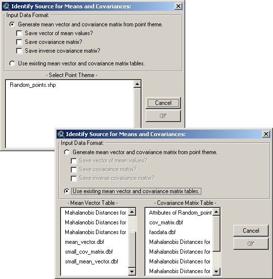
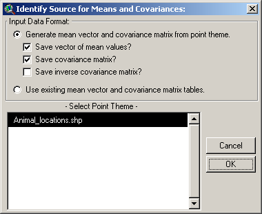
Begin the process by clicking the “Mahalanobis Distance Surface Grid” button in the View button bar. ArcView will prompt you to identify the source of your Mean Vector and Covariance Matrix. The “Identify Source for Means and Covariances” window is resizable by dragging on a corner.

Generating Means and Covariances from point theme:

This option provides a direct way to generate a landscape surface that describes how similar any point on the landscape is to a set of sample points distributed across the landscape. For a simple example, suppose that we have a set of animal locations plus a grid of elevation and slope values, and we want to identify regions on the landscape that are similar to the animal locations. This type of analysis may be useful for identifying potential habitat for an animal species.

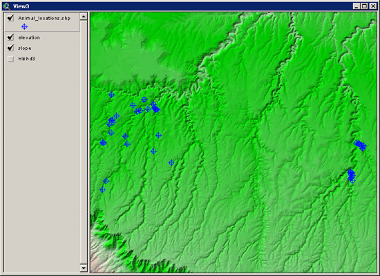
We can use the points directly to generate a vector of mean slope and elevation values for these animal locations, plus a covariance matrix for both slope and elevation values. Simply choose the first option in the “Identify Source for Means and Covariances” window and pick your point theme from the list at the bottom. You may choose to save tables of your mean vector, covariance matrix and inverse covariance matrix if you wish.

You will then be asked to identify the independent variable data grids to use with these points, and whether you wish to use exact or interpolated cell values at each point:

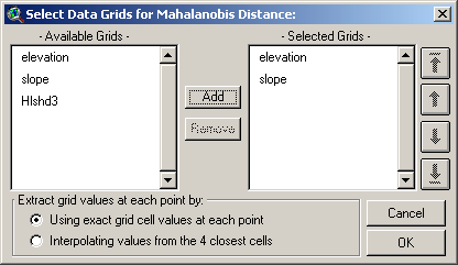
The list on the left shows all the grids available in your view and the list on the right shows all the grids that will be used in the analysis. Select one or more grids from the left and click the “Add” button to add them to the “Selected” list. If you need to reorder the selected grids (if, for example, you want to generate a mean vector or covariance matrix in a particular order), click on one of them and use the arrow buttons on the left to shift it up or down.

Exact Values vs. Interpolated Values:

You have the option to use the exact cell value for each of your point locations, or interpolated values based on the 4 closest cells to that point. For interpolated values, ArcView uses a 2-step method whereby values are interpolated first vertically and then horizontally. For example, given 4 cells around a particular location:

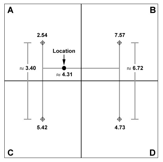
Lines are first generated between the cell centers of cells A and C, and between cells B and D, and values are interpolated along these lines at the Y-coordinate of the point location. Then a final value is interpolated along the X-axis between these two interpolated values. In this case, the interpolated value of the point is approximately 4.31, while the exact cell value of the point is 2.54.

Once you have selected your grids and point value method, click ‘OK’ to generate the Mahalanobis distance grid. When the computations are complete, the grid will be added to the view and you may then use it for any further classification or analyses.

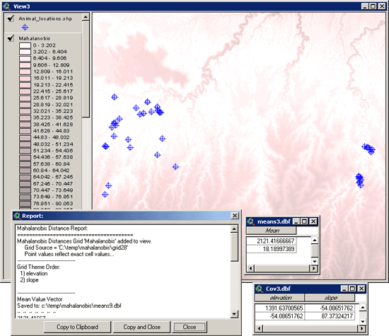
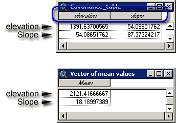
In this example, we also elected to generate tables of our Mean Value vector and Covariance matrix so both of these tables will open along with the report. The values in both tables are in the order that the original grids were entered, so here the first value in the mean vector is the Elevation mean and the second value is the Slope mean. The rows in the covariance table reflect the variables in the same order as the fields, so again Elevation is in the first row and column, and Slope is in the second row and column.

The Report Window:

You will also see a report detailing several things that may be of interest. It begins with information on the name and hard drive location of your Mahalanobis grid and the order of the independent data grids as they were included. If any output matrices were saved, the report will also include them and show where on the hard drive they were saved. Finally, the report will allow you to check if the matrix calculations worked correctly.

Recall that the Mahalanobis equation does not use the Covariance matrix directly, but rather the inverse of that matrix:

Therefore this extension must generate the inverse of the matrix before calculating the Mahalanobis distances. This extension uses the Lower/Upper Decomposition method of matrix inversion as described by Press et al. (2002).

Matrix inversion can be computationally complicated and many sources recommend checking the accuracy of the process before relying on it. The output report helps you to check that accuracy by multiplying the Covariance matrix by the Inverse covariance matrix, which should produce the Identity matrix (all 0’s except for 1’s down the diagonal):

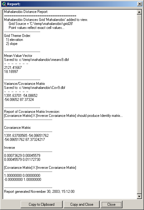
The multiplied matrix appears near the bottom of the report. Do not worry about negative 0 values; these are due to rounding issues in the computer which are an inherent problem with 32-bit operating systems. These “0” values typically have non-zero values at the 10th or greater decimal place and sometimes these values are very slightly lower than 0, forcing a “-0” value instead of a “0” value. Such matrices are still sufficiently close to perfect Identity matrices to demonstrate that the matrix inversion was successful.

Using Categorical Grids:

Categorical data do not lend themselves directly to Mahalanobis analysis. Mahalanobis values reflect how similar some set of values is to some ideal vector of values, and this ideal vector is generally assumed to be composed of the means of the variables involved. It is difficult to find the “mean” of a set of categories, and therefore they are not appropriate for Mahalanobis analysis.

However, there are aspects of categorical datasets that can be used to generate Mahalanobis distances. Clark et al. (1993) derived a numeric diversity grid from their categorical grid, where each cell value reflected the number of categories within a particular neighborhood around that cell. These data don't exactly follow a continuous distribution, but they are still reasonable as a Mahalanobis independent variable. You can generate this kind of grid using the Neighborhood Statistics function in Spatial Analyst. Generate the statistic named "Variety", which will only be available if you have an integer input grid (which is true of categorical grids).

The author has also written a tool to calculate neighborhood statistics which offers a few more options than the standard Spatial Analyst one (see Grid Tools at http://www.jennessent.com/arcview/grid_tools.htm).

Another option, also using neighborhood statistics, is to determine the proportion of the neighborhood that is composed of a particular category. You may need to generate several of these proportion grids if you want to use several categories in the Mahalanobis analysis. You can generate these category proportion grids as follows:

1. Click your "Analysis" menu, then the "Map Query..." menu item.
    

2. When the Map Query dialog opens, generate a query string querying your categorical grid for one particular category. For example, if you had a forest cover type category, you might enter:

[Cover_grid] = 4

where "4" would reflect one of the cover type categories.

3. Now you will have a "Map Query #" grid in your view, with "1" values reflecting the area represented by that category, and "0" values representing all other areas.
    

4. Open your Neighborhood Statistics tool and generate neighborhood statistics on your Map Query grid. You want to calculate the Sum, which will tell you the number of cells of that category within the specified neighborhood around each cell.
    

5. To convert this to proportions, you'll also need to find the total number of cells in that neighborhood.
    

6. Set your Analysis Environment to match your Map Query grid. Click the “Analysis” menu, then “Properties…”
    

7. In the drop-down box next to “Analysis Extent”, select your Neighborhood Sum grid.
    

8. In the drop-down box next to “Analysis Cell Size” , select your Neighborhood Sum grid.
    

9. Generate a grid of "1" values by opening the Map Calculator dialog again and entering the following calculation string:

1.AsGrid

10. Open your Neighborhood Statistics tool again, use the exact same neighborhood, and calculate the sum of your grid of "1" values. This will tell you the total number of cells within the specified neighborhood. Naturally, this value should always be ≥ the number of cells of each category within that neighborhood.
     

11. Now you have two Neighborhood Sum grids; one representing the number of cells of that category in your neighborhood, and the other representing the total number of cells in that neighborhood. Divide the Category Sum grid by the Total Sum grid and you'll get the proportion grid.
     

12. Use that Proportion grid as one of the independent grids in the Mahalanobis tool.

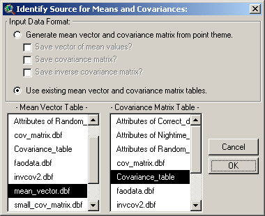
Using Existing Mean and Covariance Data:

This option allows you to use an existing mean vector and covariance matrix in your analysis rather than generating them on-the-fly from point locations. This option is useful if you have already derived your means and covariances using this extension or some other software, or if you would like to generate comparative Mahalanobis surface grids using slightly different mean vectors. Knick and Dyer (1997) describe a method of substituting a weighted mean and covariance matrix when certain input variables are better measured than others.

If you choose this option, you will need to identify the tables containing your Mean Value vector and your Covariance matrix before clicking ‘OK’:

IMPORTANT: These tables must be in the correct format for the analysis to work! Both the mean vector table and the covariance matrix table must contain only numeric values and they must be ordered correctly. The field order of the Covariance matrix table should apply to the row order of both the Covariance matrix table and the Mean Vector table:

The tool will check the tables to see if they appear to contain valid matrices before letting you continue.

Next, you will be prompted to identify your independent variable grids. These grids must be selected in the order of the matrices above, and the query window is designed to facilitate this:

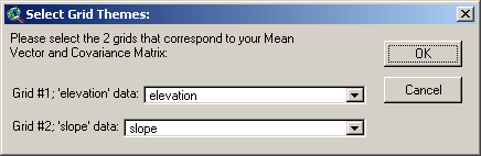
Click ‘OK’ to generate your grid. Your Mahalanobis Distance grid will be added to your view and you will see a report describing the analysis. See the discussion above on the Report window for an explanation of the report.

Mahalanobis Intro  |  Mahalanobis Description  |  Mahalanobis Chi-Square Tools  |  Mahalanobis Distances for Feature Themes  |  Mahalanobis Distances for Tables  |  Additional Mahalanobis Matrices  |  Mahalanobis References

Download Extension  |  Download Manual

Jenness Enterprises  |  ArcView Extensions  |  GIS Consultation  |  Unit Converter