General Concepts:

Mahalanobis distances provide a powerful method of measuring how similar some set of conditions is to an ideal set of conditions, and can be very useful for identifying which regions in a landscape are most similar to some “ideal” landscape.  For example, in the field of wildlife biology we might define an “ideal” landscape as that which best fits the niche of some wildlife species. Through observation, we may find that a wildlife species typically occurs within a particular elevation range, on slopes of a particular steepness, and perhaps within a certain vegetation density. Using Mahalanobis distances, we can quantitatively describe the entire landscape in terms of how similar it is to the ideal elevation, slope and vegetation density of that animal.

Moreover, Mahalanobis distances are based on both the mean and variance of the predictor variables, plus the covariance matrix of all the variables, and therefore take advantage of the covariance among variables. The region of constant Mahalanobis distance around the mean forms an ellipse in 2D space (i.e. when only 2 variables are measured), or an ellipsoid or hyperellipsoid when more variables are used.

Mahalanobis distances are calculated as:

For example, suppose we took a single observation from a bivariate population with Variable X and Variable Y, and that our two variables had the following characteristics:

and

If, in our single observation, X = 410 and Y = 400, we would calculate the Mahalanobis distance for that single value as:

Therefore, our single observation would have a distance of 1.825 standardized units from the mean (mean is at X = 500, Y = 500).

If we took many such observations, graphed them and colored them according to their Mahalanobis values, we can see the elliptical Mahalanobis regions come out. For example, the cloud of data points to the right are randomly generated from the bivariate population described above:

The points are actually distributed along two primary axes:

If we calculate Mahalanobis distances for each of these points and shade them according to their distance value, we see clear elliptical patterns emerge:

We can also draw actual ellipses at regions of constant Mahalanobis values:

One interesting feature to note from this figure is that a Mahalanobis distance of 1 unit corresponds to 1 standard deviation along both primary axes of variance.

Chi-Square P-values:

Mahalanobis distances are occasionally converted to Chi-square p-values for analysis (see Clark et al. 1993). When the predictor variables are normally distributed, the Mahalanobis distances do follow the Chi-square distribution with n-1 degrees of freedom (where n = # of habitat variables; 2 in the example above). However, Farber and Kadmon (2003) warn that wildlife habitat variables often fail to meet the assumption of normality. In cases where the predictor variables are not normally distributed, the conversion to Chi-square p-values serves to recode the Mahalanobis distances to a 0-1 scale. Mahalanobis distances themselves have no upper limit, so this rescaling may be convenient for some analyses.

In general, the p-value reflects the probability of seeing a Mahalanobis value as large or larger than the actual Mahalanobis value, assuming the vector of predictor values that produced that Mahalanobis value was sampled from a population with an ideal mean (i.e. equal to the vector of mean predictor variable values used to generate the Mahalanobis value). P-values close to 0 reflect high Mahalanobis distance values and are therefore very dissimilar to the ideal combination of predictor variables. P-values close to 1 reflect low Mahalanobis distances and are therefore very similar to the ideal combination of predictor variables. The closer the p-value is to 1, the more similar that combination of predictor values is to the ideal combination.

Applications to Landscape Analysis:

A nice feature of ArcView Spatial Analyst is that we can use actual grids in the Mahalanobis Distance equation rather than numbers, so we can input a vector of habitat grids in place of the vector of input values. We still need the vector of mean values and the covariance matrix, but Spatial Analyst will treat each of these values as an individual landscape-scale grid of that value, and therefore the mathematical functions in Spatial Analyst will work correctly and produce a final grid of Mahalanobis values. Due to a limitation in Spatial Analyst, however, we are limited to 8 input grids for this analysis. Spatial Analyst v. 9 is supposed to fix this limitation.

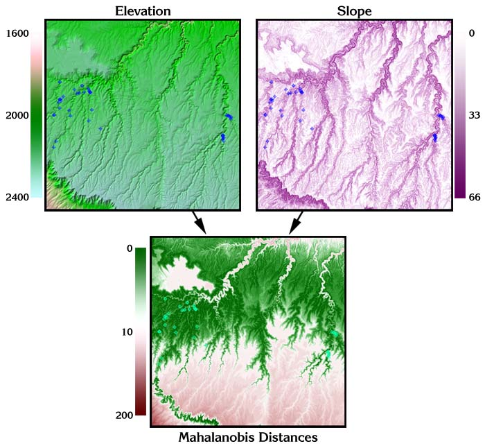
For example, suppose we have a grid of elevation values and a grid of slope values, and we are interested in identifying those regions on the landscape that have similar slopes and elevations to a mean slope and elevation preferred by some species of interest. Furthermore, we want to analyze the slope and elevations in combination so that if our species likes steep slopes at low elevations but shallow slopes at high elevations, then we won’t inadvertently select steep slopes at high elevations or shallow slopes at low elevations.

Assume that the niche of our species of interest can be described in terms of Elevation and Slope with the following parameters:

We can then enter the Elevation and Slope grids directly into the Mahalanobis equation to produce a Mahalanobis grid:

Additional Reading:

The author recommends Clark et al. (1993), Knick & Dyer (1997), and Farber & Kadmon (2002) for a few good papers illustrating the use of Mahalanobis distances in ecological applications. For anyone interested in the details of matrix algebra and computational/statistical algorithms, the author recommends Conover (1980), Neter et al. (1990), Golub and Van Loan (1996), Draper and Smith (1998), Meyer (2000) and Press et al. (2002).

Mahalanobis Intro  |   Generating Mahalanobis Grids  |  Mahalanobis Chi-Square Tools  |  Mahalanobis Distances for Feature Themes  |  Mahalanobis Distances for Tables  |  Additional Mahalanobis Matrices  |  Mahalanobis References

Download Extension  |  Download Manual

Jenness Enterprises  |  ArcView Extensions  |  GIS Consultation  |  Unit Converter