Jenness Enterprises - Statistical Distributions; Quantile Functions

Mexican Spotted Owl, stretching...

In general, the Quantile Functions (sometimes referred to as Inverse Density Functions or Percent Point Functions) return the Value X at which P(X) = [specified cumulative probability], given that particular distribution.

Distributions
Beta	Chi Square	Logistic	Poisson
Binomial	Exponential	LogNormal	Student's T
Cauchy	F	Normal	Weibull

IDF_Beta: This function takes the specified probability and returns the value X, such that P(X) = P-value, given the Beta distribution with the two specified Shape parameters. Because the formula for this function does not exist in a closed form, it must be computed numerically. This script arrives at the X-value through an iterative process, repeatedly testing X-values with the CDF_Beta function until it arrives at P value that is within 1x10^-12 units from the specified P-value (this usually takes between 30-60 iterations).
a) Parameters:
1. P-value: Number (0 >= p >= 1)
2. Shape1: Number > 0
3. Shape2: Number > 0
b) Usages:
1. From "Probability Distribution Calculator", select "Quantile (IDF)" and Beta distribution.
2. (Avenue): theProb = av.Run("Jennessent.DistFunc”, {“IDF_Beta”, {P-value, Shape1, Shape2}})
3. (Avenue): theProb = av.Run("Jennessent.TableDistFunc”, {“IDF_Beta”, {P-value, Shape1, Shape2}})
4. (Avenue): theProb = av.Run("Jennessent.IDF_Beta", {P-value, Shape1, Shape2})
c) Function: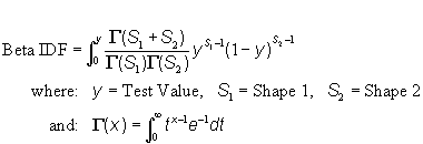

IDF_Binomial: This function takes the specified probability and returns the value X such that the Probability of getting (X – 1) successes <= the Specified Probability. This function takes an iterative approach to finding the correct X value, repeatedly trying different values of X until it reaches the correct one. This iterative process rarely takes more than 25 repetitions.
a) Parameters:
1. P-value: Number (0 >= p >= 1)
2. # Trials: Integer >= 2, # Successes
3. Probability of Success: Number (0 >= p >= 1)
b) Usages:
1. From "Probability Distribution Calculator", select "Quantile (IDF)" and Binomial distribution.
2. (Avenue): theProb = av.Run("Jennessent.DistFunc”, {“IDF_Binomial”, {P-value, #Trials, Probability of Success}})
3. (Avenue): theProb = av.Run("Jennessent.TableDistFunc”, {“IDF_Binomial”, {P-value, #Trials, Probability of Success}})
4. (Avenue): theProb = av.Run("Jennessent.IDF_Binomial", {P-value, #Trials, Probability of Success})
c) Function:

IDF_Cauchy: This function takes the specified probability and returns the value X, such that P(X) = P-value, given the Cauchy distribution with the specified location and scale parameters. The Standardized Cauchy distribution has Location = 0 and Scale = 1.
a) Parameters:
1. P-value: Number (0 >= p >= 1)
2. Location: Number
3. Scale: Number > 0
b) Usages:
1. From "Probability Distribution Calculator", select "Quantile (IDF)" and Cauchy distribution.
2. (Avenue): theProb = av.Run("Jennessent.DistFunc”, {“IDF_Cauchy”, {P-value, Location, Scale}})
3. (Avenue): theProb = av.Run("Jennessent.TableDistFunc”, {“IDF_Cauchy”, {P-value, Location, Scale}})
4. (Avenue): theProb = av.Run("Jennessent.IDF_Cauchy", {P-value, Location, Scale})
c) Function:

IDF_ChiSquare: This function takes the specified probability and returns the value X, such that P(X) = P-value, given the Chi-Square distribution with the specified Degrees of Freedom. Because the formula for this function does not exist in a closed form, it must be computed numerically. This script arrives at the X-value through an iterative process, repeatedly testing X-values with the CDF_ChiSquare function until it arrives at P value that is within 1x10 -12 units from the specified P-value (this usually takes between 30-60 iterations). The Chi-Square distribution results when v (where v = Degrees of Freedom) independent variables with standard normal distributions are squared and summed (Croarkin & Tobias, Date unknown).
a) Parameters:
1. P-value: Number (0 >= p >= 1)
2. Degrees of Freedom: Number > 0
b) Usages:
1. From "Probability Distribution Calculator", select "Quantile (IDF)" and Chi Square distribution.
2. (Avenue): theProb = av.Run("Jennessent.DistFunc”, {“IDF_ChiSquare”, {P-value, DF}})
3. (Avenue): theProb = av.Run("Jennessent.TableDistFunc”, {“IDF_ChiSquare”, {P-value, DF}})
4. (Avenue): theProb = av.Run("Jennessent.IDF_ChiSquare", {P-value, DF})
c) Function: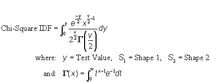

IDF_Exp: This function takes the specified probability and returns the value X, such that P(X) = P-value, given the Exponential distribution with the specified mean. This script uses the 1-parameter version of the equation (i.e. assuming Location = 0). The Standard Exponential Distribution is that which has Mean = 1.
a) Parameters:
1. P-value: Number (0 >= p >= 1)
2. Mean: Number > 0
b) Usages:
1. From "Probability Distribution Calculator", select "Quantile (IDF)" and Exponential distribution.
2. (Avenue): theProb = av.Run("Jennessent.DistFunc”, {“IDF_Exp”, {P-value, Mean}})
3. (Avenue): theProb = av.Run("Jennessent.TableDistFunc”, {“IDF_Exp”, {P-value, Mean}})
4. (Avenue): theProb = av.Run("Jennessent.IDF_Exp", {P-value, Mean})
c) Function:

IDF_F: This function takes the specified probability and returns the value X, such that P(X) = P-value, given the F distribution with the specified Degrees of Freedom. Because the formula for this function does not exist in a closed form, it must be computed numerically. This script arrives at the X-value through an iterative process, repeatedly testing X-values with the CDF_F function until it arrives at P value that is within 1x10^-12 units from the specified P-value (this usually takes between 30-60 iterations). The F distribution is the ratio of two Chi Square distributions with ratios v₁ and v₂ respectively.
a) Parameters:
1. P-value: Number (0 >= p >= 1)
2. 1st Degrees of Freedom: Number > 1
3. 2nd Degrees of Freedom: Number > 1
b) Usages:
1. From "Probability Distribution Calculator", select "Quantile (IDF)" and F distribution.
2. (Avenue): theProb = av.Run("Jennessent.DistFunc”, {“IDF_F”, {P-value, DF1, DF2}})
3. (Avenue): theProb = av.Run("Jennessent.TableDistFunc”, {“IDF_F”, {P-value, DF1, DF2}})
4. (Avenue): theProb = av.Run("Jennessent.IDF_F", {P-value, DF1, DF2})
c) Function: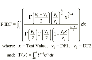

IDF_Logistic: This function takes the specified probability and returns the value X, such that P(X) = P-value, given the Logistic distribution with the specified mean and scale parameters.
a) Parameters:
1. P-value: Number (0 >= p >= 1)
2. Mean: Number
3. Scale: Number > 0
b) Usages:
1. From "Probability Distribution Calculator", select "Quantile (IDF)" and Logistic distribution.
2. (Avenue): theProb = av.Run("Jennessent.DistFunc”, {“IDF_Logistic”, {P-value, Mean, Scale}})
3. (Avenue): theProb = av.Run("Jennessent.TableDistFunc”, {“IDF_Logistic”, {P-value, Mean, Scale}})
4. (Avenue): theProb = av.Run("Jennessent.IDF_Logistic", {P-value, Mean, Scale})
c) Function:

IDF_LogNormal: This function takes the specified probability and returns the value X, such that P(X) = P-value, given the LogNormal distribution with the specified mean and scale parameters. Because the formula for this function does not exist in a closed form, it must be computed numerically. This script arrives at the X-value through an iterative process, repeatedly testing X-values with the CDF_LogNormal function until it arrives at P value that is within 1x10^-12 units from the specified P-value (this usually takes between 30-60 iterations). A LogNormal distribution occurs when natural logarithms of variable X are normally distributed. The Standard LogNormal Distribution is that with Mean = 0 and Scale = 1. The 2-Parameter LogNormal Distribution is that with Mean = 0.
a) Parameters:
1. P-value: Number (0 >= p >= 1)
2. Mean: Number > 0
3. Scale: Number > 0
b) Usages:
1. From "Probability Distribution Calculator", select "Quantile (IDF)" and LogNormal distribution.
2. (Avenue): theProb = av.Run("Jennessent.DistFunc”, {“IDF_LogNormal, {P-value, Mean, Scale}})
3. (Avenue): theProb = av.Run("Jennessent.TableDistFunc”, {“IDF_LogNormal, {P-value, Mean, Scale}})
4. (Avenue): theProb = av.Run("Jennessent.IDF_LogNormal", {P-value, Mean, Scale})
c) Function:

IDF_Normal: This function takes the specified probability and returns the value X, such that P(X) = P-value, given the Normal distribution with the specified mean and standard deviation. Because the formula for this function does not exist in a closed form, it must be computed numerically. This script arrives at the X-value through an iterative process, repeatedly testing X-values with the CDF_Normal_Simpsons function until it arrives at P value that is within 1x10^-12 units from the specified P-value (this usually takes between 30-60 iterations). Furthermore, there is no closed formula for calculating the Normal cumulative distribution function, so this script uses the Simpson’s approximation method (Stewart 1998, p. 421-424) to calculate a highly accurate estimate (accuracy to > 12 decimal places). The Standard Normal Distribution is that with Mean = 0 and Standard Deviation = 1.
a) Parameters:
1. P-value: Number (0 >= p >= 1)
2. Mean: Number
3. Standard Deviation: Number > 0
b) Usages:
1. From "Probability Distribution Calculator", select "Quantile (IDF)" and Normal distribution.
2. (Avenue): theProb = av.Run("Jennessent.DistFunc”, {“IDF_Normal_Simpsons, {P-value, Mean, St. Dev.}})
3. (Avenue): theProb = av.Run("Jennessent.TableDistFunc”, {“IDF_Normal_Simpsons, {P-value, Mean, St. Dev.}})
4. (Avenue): theProb = av.Run("Jennessent.IDF_Normal_Simpsons", {P-value, Mean, St. Dev.})
c) Function:

IDF_Poisson: This function takes the specified probability and returns the value X such that the Probability of getting (X – 1) events <= the Specified Probability. This function takes an iterative approach to finding the correct X value, repeatedly trying different values of X until it reaches the correct one.
a) Parameters:
1. P-value: Number (0 >= p >= 1)
2. Mean: Number > 0
b) Usages:
1. From "Probability Distribution Calculator", select "Quantile (IDF)" and Poisson distribution.
2. (Avenue): theProb = av.Run("Jennessent.DistFunc”, {“IDF_Poisson, {#P-value, Mean}})
3. (Avenue): theProb = av.Run("Jennessent.TableDistFunc”, {“IDF_Poisson, {P-value, Mean}})
4. (Avenue): theProb = av.Run("Jennessent.IDF_Poisson", {P-value, Mean})
c) Function: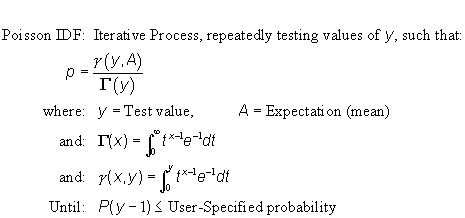

IDF_StudentsT: This function takes the specified probability and returns the value X, such that P(X) = P-value, given the Student’s T distribution with the specified Degrees of Freedom. Because the formula for this function does not exist in a closed form, it must be computed numerically. This script arrives at the X-value through an iterative process, repeatedly testing X-values with the CDF_StudentsT function until it arrives at P value that is within 1x10^-12 units from the specified P-value (this usually takes between 30-60 iterations). A Student’s T distribution with 1df is a Cauchy Distribution, and it approaches a Normal distribution when DF>30. Various sources recommend using the Normal distribution if DF>100.
a) Parameters:
1. P-value: Number (0 >= p >= 1)
2. Degrees of Freedom: Number > 0
b) Usages:
1. From "Probability Distribution Calculator", select "Quantile (IDF)" and Student’s T distribution.
2. (Avenue): theProb = av.Run("Jennessent.DistFunc”, {“IDF_StudentsT, {P-value, DF}})
3. (Avenue): theProb = av.Run("Jennessent.TableDistFunc”, {“IDF_StudentsT, {P-value, DF}})
4. (Avenue): theProb = av.Run("Jennessent.IDF_StudentsT", {P-value, DF})
c) Function: The IDF_StudentsT T Function is dependent on whether the test value is positive or negative:

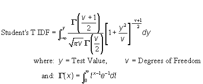IDF_Weibull: This function takes the specified probability and returns the value X, such that P(X) = P-value, given the Weibull distribution with the specified Location, Scale and Shape parameters. The Standardized Weibull Distribution is that with Location = 0 and Scale = 1. The 2-Parameter Weibull Distribution is that with Location = 0.
a) Parameters:
1. P-value: Number (0 >= p >= 1)
2. Location: Number
3. Scale: Number > 0
4. Shape: Number > 0
b) Usages:
1. From "Probability Distribution Calculator", select "Quantile (IDF)" and Weibull distribution.
2. (Avenue): theProb = av.Run("Jennessent.DistFunc”, {“IDF_Weibull, {P-value, Location, Scale, Number}})
3. (Avenue): theProb = av.Run("Jennessent.TableDistFunc”, {“IDF_Weibull, {P-value, Location, Scale, Number}})
4. (Avenue): theProb = av.Run("Jennessent.IDF_Weibull", {P-value, Location, Scale, Number})
c) Function:

Back to Statistics/Distributions | Summary Statistics | Probability Calculators | References

Calculating Summary Statistics with Avenue

Discussion of Distribution Functions:
Probability Density Functions | Cumulative Distribution Functions | Quantile Functions

Download Statistics Extension Manual (Adobe PDF, version 5)

Please visit Jenness Enterprises ArcView Extensions site for more ArcView Extensions and other software by the author. We also offer customized ArcView-based GIS consultation services to help you meet your specific data analysis and application development needs.