![]()
![]()
![]()
![]()
![]()
![]()
![]()

NAME: Nearest Features v. 3.8b (Click Name to Download)
AKA: NearFeat.avx
Last Modified: February 15, 2007
TITLE: Nearest Features, with Distances and Bearings (v. 3.8b)
TOPICS: ArcView 3.x, Nearest Feature, Distance, Bearing, Azimuth, View, Analysis, Tools, Centroid, Closest Edge, Maximum Search Radius, Length, Great Circle, Geodesic
AUTHOR: Jeff Jenness
Wildlife Biologist, GIS Analyst
Jenness Enterprises
3020 N. Schevene Blvd.
Flagstaff, AZ 86004
DESCRIPTION: This extension creates a new button on the VIEW toolbar which enables you to identify which comparison features are nearest to some set of input features you are interested in. Begin by selecting an Input theme containing the features of interest, then either a single or multiple comparison themes containing features you want to compare. The extension then steps through each feature in the input theme and finds which feature, out of all the comparison themes, is closest to it. The extension then creates a results table (described below) containing various user-selected fields such as distance and bearing between features. Optionally, you can request lines to be drawn connecting each input feature with that closest comparison feature and save these lines as a Polyline shapefile.
Multiple Levels of Nearness: This extension allows you to calculate the 1st, 2nd, … nth closest comparison features to each input feature. Distance, bearing, and graphic lines can be calculated for each level of nearness as well.
Centroids vs. Closest Edges: If desired, this extension can calculate the distance and bearing between the centroids of the closest features as well as the distance and bearing between the closest edges of those features. For example, if a point theme and a polygon theme are used in the analysis, then this extension will determine what point on the edge of the closest polygon (not necessarily a vertex) is closest to the input point. If the features intersect or if one lies within the other, then you have the option to either set the distances to zero or not, thereby allowing you to calculate the closest distances to the edge from features enclosed by other features. You can request that graphics be drawn connecting the centroids and/or the closest edges of the closest features and you have the option to save these connecting lines into a separate Polyline shapefile.
Closest Features Within a Single Theme: You can select a single theme to act as both the input theme AND comparison theme, in which case this extension will measure the distances from each feature in that theme to all the other features in that theme. It will NOT measure the distance to itself, so you will not get a bunch of zero distances.
All or only selected records: You can either use all the features in each of the themes for the analysis or only a selected subset of features. If any features in a particular theme (input or comparison themes) are selected, then only those selected features in that theme will be used in the analysis. If no features in a theme are selected, then all features in that theme will be used in the analysis.
Great Circle Distances: Offers the option to calculate distances and bearings based on geodesic curves reaching over the surface of the planet. This option is offered only if both input and comparison themes are point themes.
Projected vs. Unprojected Views: If your original data are in Lat/Long coordinates (the Geographic Projection) and your View has been projected, then you have the option of calculating RESULTS data based on either the Geographic Projection or your View Projection. The choice of projections can affect which features are considered nearest, as well as affecting distances, bearings and coordinates.
OUTPUT:
Results Table: Upon completion, you will have a results table containing some or all of the following fields. These fields are chosen by you and the field will not be calculated if you do not want it. The symbol "#" in the following description refers to the nearness of that comparison feature. For example, if you want to identify only the ID of the five nearest features, then the Results table will have six fields, labeled [input ID], [1_ID], [2_ID], [3_ID], [4_ID], and [5_ID]. Optionally, you can request the Results table to be joined with the input DBF file. The field names will all begin with the letter “n” so that the table can be easily exported into other software.
- ID: Input theme ID, taken from the Input theme DBF file. Each Input feature is identified in the result table allowing it to be linked back to the original Input theme shapefile. The name of this field is the name of the selected Input ID field.
Polyline Shapefile: If you choose to save your connection lines as a polyline shapefile, then each connection line will be saved as a separate polyline. The shapefile will include only those connection lines that you specify in the "Additional Options" dialog box. This shapefile will be added to your view as a new theme. The Feature Attribute Table for the shapefile will contain the following fields:
- ID: Input theme ID, taken from the Input theme DBF file. Each Input feature is identified in the result table allowing it to be linked back to the original Input theme shapefile. The name of this field is the name of the selected Input ID field.
- Unique_ID: A unique numeric ID value for each polyline in the shapefile.
- near_level: The nearness level of the comparison feature. For example, if this was the second closest feature to the input feature, this field would have the value "2".
- cent_edge: Specifies whether this connection line connects the Centroids or the Nearest Edges of the respective features. All values in this field will be either "Centroids" or "Edges".
- comp_theme: (Only if requested) The theme name of the Comparison Theme that this particular comparison feature came from. Remember that there can be multiple comparison themes in a single analysis.
- comp_ID: Comparison theme ID, taken from the specified comparison theme ID Field.
- distance: The length of the connection line.
- bearing: The compass bearing from the Input feature to the Comparison feature. This bearing is calculated from the X-Y coordinate system of the projection used in the analysis.
- Start_X: The X-coordinate of the starting point of the connection line.
- start_Y: The Y-coordinate of the starting point of the connection line.
- end_X: The X-coordinate of the end point of the connection line.
- end_Y: The Y-coordinate of the end point of the connection line.
REQUIRES: This extension requires a minimum of one feature theme (Point, Line or Polygon theme) present in a view if you want to find which features within a single theme are closest to each other. Otherwise, a minimum of two feature themes are needed; one to act as the 'Input' theme and at least one 'Comparison' theme.
This extension also requires that the file "avdlog.dll" be present in the ArcView/BIN32 directory (or $AVBIN/avdlog.dll) and that the Dialog Designer extension be available in the ArcView/ext32 directory, which they almost certainly are if you're running AV3.1 or higher. You don't have to load the Dialog Designer; it only has to be available. If you are running AV 3.0a, you can download the appropriate files for free from ESRI at:
http://support.esri.com/index.cfm?fa=downloads.patchesServicePacks.viewPatch&PID=25&MetaID=483
Recommended Citation Format: For those who wish to cite this extension, the author recommends something similar to:
Jenness, J. 2004. Nearest features (nearfeat.avx) extension for ArcView 3.x, v. 3.8a. Jenness Enterprises. Available at: http://www.jennessent.com/arcview/nearest_features.htm.
Please let me know if you cite this extension in a publication (jeffj@jennessent.com). I will update the citation list to include any publications that I am told about (see Citations).
Revisions described at bottom of page:
![]()
GENERAL INSTRUCTIONS:
1) Begin by placing the "NearFeat.avx" file into the ArcView extensions directory (../../Av_gis30/ArcView/ext32/).
2) After starting ArcView, Load the extension by clicking on File à Extensions… , scrolling down through the list of available extensions, and then clicking on the checkbox next to the extension called "Nearest Features, v. 3.8a"
3) Select Input Theme: Begin by clicking on the
![]() button. This brings up the Input Theme dialog box:
button. This brings up the Input Theme dialog box:
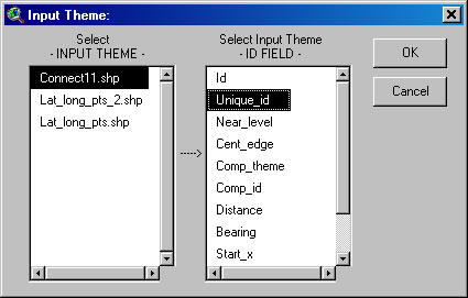
The – INPUT THEME – list shows all of the Feature Themes (those themes made of Points, Lines or Polygons) in the view. Once you select the input theme of interest, the –ID FIELD – list becomes active and shows a list of all the fields in the input theme’s Feature Attribute Table. You must select a field that contains a unique identifier for each feature. This identifier allows your RESULTS table to be joined with your input theme Feature Table, and it also necessary for you to know which input feature is compared with the various comparison features.
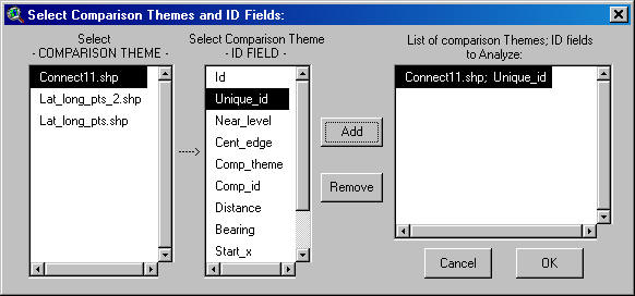
4) Select Comparison Themes and ID Fields: After the Input Theme has been selected, select either a single or multiple comparison themes. This dialog box works the same as the Input Theme dialog box except that you can add multiple Theme/ID Field combinations to the analysis. Notice that you can also include the Input Theme as a comparison theme. In this case, the program will compare all features with the input feature EXCEPT that input feature. In other words, this program will not compare a feature with itself. The closest feature to any feature will always be itself, but that information is rarely what users are looking for.
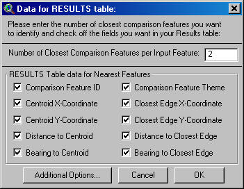
5) Select Data to be included in RESULTS table: Select how many Nearest Features you want to identify from the Comparison Features for each input feature, and then select which of the 10 possible data fields you want calculated for each input feature. Note that this can produce a lot of fields in the RESULTS table. If you want to calculate all 10 fields on the five closest Comparison Features, the Results Table will have 51 fields in it.
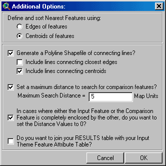
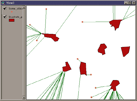
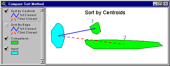
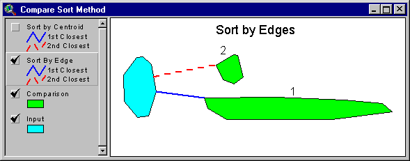
a. Define and sort Nearest Features using: This option allows you to select your nearest features based on whether the Edges or Centroids of the respective Comparison features are nearest to that Input feature. Often a particular feature may be considered “nearest” by one definition but not by the other. For example, the illustration below shows a situation where two comparison features are ranked differently depending on whether centroids or edges are used:
b. Generate a Polyline Shapefile of connecting lines? This option produces a new polyline theme in your view representing all lines connecting either the centroids or the nearest edges of the respective features. The feature Attribute Table for this theme will include ID values of the Input and Comparison feature, the distance and bearing from the Input to the Comparison feature, whether the line connects Centroids or Edges, and the coordinates of the start and end points of the lines (see Description of Polyline Shapefile for specific fields).
c. Set a maximum distance to search for comparison features? This option can significantly increase the processing speed by restricting the number of comparison features ArcView analyzes. If you don't select this option, then ArcView will search all comparison features to find the nearest ones. If you set a maximum search distance, then ArcView will only analyze those comparison features within that distance.
This option requires you to make an estimate of the maximum distance that will capture all the desired comparison features. You can usually make a reasonable estimate by using the "Measure" tool in your view to measure the largest distance between features. This extension will warn you at the end of the processing if you entered a distance that was too low (i.e. if your distance caused some input features to not have any comparison features). Also, the Results table will get null numbers for these occasions (which are different than zeros) and the table will therefore have empty cells in it.ATTENTION: Another Tip To Speed Operations: Under certain circumstances you may be able to make your analysis calculate more quickly. This fast-mode operation will be most useful for Nearest Features analysis with many polygons and/or polygons with high numbers of vertices. It takes a lot of extra time calculating the actual points on the polygons that are nearest to each other. Therefore you can reduce the calculation time by avoiding these calculations. Select NO MORE than the following options from your “Data for RESULTS Table:” dialog above:
- Comparison Feature ID
- Comparison Feature Theme
- Distance to Closest Edge
- “Set Distances to Zero” should be CHECKED.
- Do NOT select any graphics (You will be asked about graphics shortly).
- The “Join Tables” option will have no effect on calculation time.
d. Set Distance Values to 0? You have the option to set distances equal to zero if one feature is enclosed by another. Essentially the distances ARE zero in this case, and so this option should usually be checked. However, in some cases you may need to know the distance to the nearest edges of a polygon that encloses your input features, and in such a case you can turn this option off.
e. Join your RESULTS table with your Input Theme Feature Attribute Table? By default you will end up with a RESULTS table labeled "Closest Features to [Input Theme Name]", but you have the option here to have the RESULTS table joined to the Input Feature Table automatically.
7) If your view is projected, then the extension will assume that your actual data are in Latitude/Longitude coordinates. If so, then distances between them will likely be very inaccurate because Decimal Degrees make poor distance units. In this case the extension will ask you whether you would prefer to calculate distance and azimuth values according to the coordinate system of the View projection. If both your Input and Comparison themes are Point themes, then you will also have the option to calculate distances based on geodesic curves (also known as great circle distances). This choice can have dramatic differences on distances, bearings and edge coordinates, and even on which features are considered “nearest.”
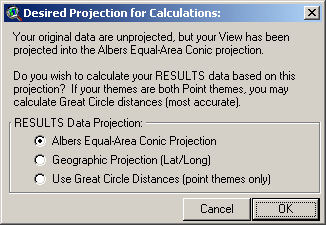
Distances measured in “degrees” become especially problematic the farther you get from the equator, since longitudinal degrees are not the same as latitudinal degrees. The author recommends that the user calculate the RESULTS data based on the View Projection rather than the Geographic projection, unless the user has some specific reason to need the results to be based on latitude and longitude coordinates.
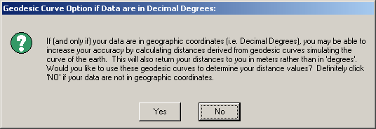
If your view is not projected, AND if both your Input and Comparison themes are Point themes, AND if it appears that your data are in lat/long coordinates (i.e. all X-coordinates are between -180 and 180 and all Y-coordinates are between -90 and 90) then you will still have the option to calculate distances based on geodesic curves. You will be asked if you would like to use geodesic curves in the following window:
Discussion of Geodesic Curves:
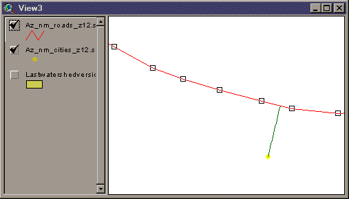
These geodesic distances are really the only way to get consistently accurate distance measures when your route goes over significant portions of the earth. This method is more accurate than using an equidistant map projection because such projections are only accurate between specific points. These geodetic curves allow us to determine distances between any two points on the globe.
For example, the following image illustrates a long-distance migration route for a hypothetical bird. It may fly in a straight line from Uruguay to Alaska, but only a equidistant projection specifically set for this route can produce accurate values for distance and azimuth. Geodesic curves do not rely on particular projections because they model the actual shape of the world in 3 dimensions. They do, however, depend on a spheroidal model, and this extension uses the WGS-80 spheroid for all geodesic calculations.
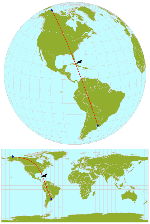
If you do use the Geodesic Curve option, then distances will always be reported in meters
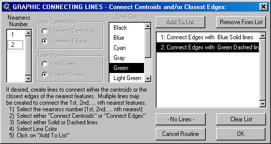
8) Add Connection Lines: You have the option to create graphic connecting lines to connect each of the Input Features with it's respective nearest Comparison Features. In this dialog box you begin by selecting the "Nearness Number", reflecting the 1st, 2nd, … nth Comparison Feature to draw lines to. Then checks whether you want to connect the centroids of the features or the closest edges, and then whether you want the lines to be solid or dashed. Finally pick a color for the line and add it the list. This extension will create graphic lines for all the Line/Color/Style combinations in the list.
This dialog box is resizable, so you can stretch it if you cannot read the entire description in the list.
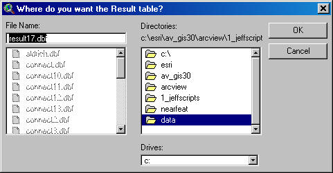
9) Specify Hard Drive Location to save your output: You will be prompted to specify a location on the hard drive to save your RESULTS table and your Connecting Lines Shapefile, if requested. These are standard ArcView Dialog Boxes and should be familiar to most users. The RESULTS table is a permanent table and will not be deleted when ArcView is shut down.
![]()
Troubleshooting: If you encounter some strange crash, please click the menu item “Check ‘Nearest Features’ Scripts” in either the View or Project Help menu. Click this as soon as you are able to following the crash. With any luck, that function will generate a report with enough information for the author to find and fix the problem.
Enjoy! Please contact the author if you have problems or find bugs.
Jeff Jenness jeffj@jennessent.com
3020 N. Schevene Blvd.
Flagstaff, AZ 86004
USA
![]()
Please visit Jenness Enterprises ArcView Extensions site for more ArcView Extensions and other software by the author. We also offer customized ArcView-based GIS consultation services to help you meet your specific data analysis and application development needs.
![]()
![]()
This extension has been cited by:
| K. Johnson, B.H. Smith, G. Sadoti, T.B. Neville,
and P. Neville. 2004. Habitat use and nest site selection by nesting Lesser Prairie-Chickens in southeastern New Mexico. Southwestern Naturalist 49(3):334-343. |
Abstract: Lesser prairie-chickens (Tympanuchus pallidicinctus) occur in shinnery oak (Quercus havardii) and sand sagebrush (Artemisia filifolia) grassland habitats in New Mexico, Texas, Oklahoma, Kansas, and Colorado. Range-wide population reductions since the 1800s have been attributed to habitat loss, especially of nesting habitat. Using radio-telemetry and a vegetation map of the study area, we investigated habitat use by lesser prairie-chicken hens during the nesting season in herbicide-treated and untreated pastures (each about 1,000 ha in size). Herbicide treatment was effective in reducing shinnery oak cover. The most common vegetation types in hen home ranges were those dominated by shinnery oak. Hens were detected more often than randomly in or near untreated pastures. Although hens were detected in both treated and untreated habitats, 13 of 14 nests were located in untreated pastures, and all nests were located in areas dominated by shinnery oak. Areas immediately surrounding nests had higher shrub composition than the surrounding pastures. This study suggests that herbicide treatment to control shinnery oak might adversely impact nesting lesser prairie-chickens.
| Mennill, D. J. and Ratcliffe, L. M. 2004. Nest cavity orientation in black-capped chickadees Poecile atricapillus : do the acoustic properties of cavities influence sound reception in the nest and extra-pair matings? J. Avian Biol. 35: 477-482. (Available here). |
Abstract: Birds that nest in cavities may regulate nest microclimate by orienting their nest entrance relative to the sun or prevailing winds. Alternatively, birds may orient their nest entrance relative to conspecific individuals around them, especially if the acoustic properties of cavities permit nesting birds to better hear individuals in front of their nest. We measured the cavity entrance orientation of 132 nests and 234 excavations in a colour-banded population of black-capped chickadees Poecile atricapillus for which the reproductive behaviour of nesting females was known. Most chickadees excavated cavities in rotten birch Betula papyrifera , aspen Populus tremuloides and maple Acer saccharum. Nest cavities showed random compass orientation around 3608 demonstrating that chickadees do not orient their cavities relative to the sun or prevailing winds. We also presented chickadees with nest boxes arranged in groups of four, oriented at 908 intervals around the same tree. Nests constructed in these nest box quartets also showed random compass orientation. To test the acoustic properties of nest cavities, we conducted a sound transmission experiment using a microphone mounted inside a chickadee nest. Re-recorded songs demonstrate that chickadee nest cavities have directional acoustic properties; songs recorded with the cavity entrance oriented towards the loudspeaker were louder than songs recorded with the cavity entrance oriented away from the loudspeaker. Thus, female chickadees, who roost inside their nest cavity in the early morning during their fertile period, should be better able to hear males singing the dawn chorus in front of their nest cavity. Using GIS analyses we tested for angular-angular correlation between actual nest cavity orientation and the azimuth from the nest tree to the territories and nest cavities of nearby males. In general, nest cavity entrances showed no angular-angular correlation with neighbourhood territory features. However, among birds who followed a mixed reproductive strategy and nested in the soft wood of birch and aspen trees, nest cavity entrances were oriented towards their extra-pair partners. We conclude that nest cavity orientation in birds may be influenced by both ecological and social factors.
| Mennill DJ, Ramsay SM, Boag PT, & Ratcliffe LM (2004) Patterns of extrapair mating in relation to male dominance status and female nest placement in black-capped chickadees. Behavioral Ecology 15:757-765. (Available here). |
Abstract: In sexually promiscuous animals, females may benefit by nesting close to the edge of their partner’s territory to facilitate extrapair copulations. In the present study, we describe the extrapair mating system of black-capped chickadees, Poecile atricapillus, and test whether nest locations are influenced by conspecific attraction to extrapair partners. We conducted a spatial analysis of female mating strategies by using microsatellite paternity analysis in conjunction with geographic information system (GIS) analysis of nest and territory locations. Extrapair offspring comprised 52 of 351 offspring (14.8%) and were present in 19 of 57 broods (33.3%). Females paired to males with low dominance status in the previous winter’s flock hierarchy were more likely to engage in a mixed reproductive strategy than were females paired to males with high dominance status. Females had extrapair copulations and extrapair fertilizations with high-ranking males more often than with low-ranking males. Not all extrapair copulations resulted in extrapair fertilizations. Females constructed their nests within 16.8 6 1.0 m of the edge of their partner’s territory, significantly closer to the edge of their nearest neighbor’s territory than to the center of their own partner’s territory. Extrapair males usually shared territory boundaries with cuckolded males. Females paired to low-ranking males constructed nests near the territory edges of neighboring high-ranking males. However, females did not have extrapair copulations with the neighbor nearest to their nest or even with the high-ranking neighbor nearest to their nest. We conclude that conspecific attraction to neighbors may influence nesting location in black-capped chickadees; however, it does not operate by facilitating extrapair copulations. Key words: black-capped chickadee, conspecific attraction, extrapair copulations, extrapair fertilizations, female choice, male dominance rank, nest location, Poecile atricapillus. [Behav Ecol 15:757–765 (2004)]
![]()
3.1: Fixes a problem with drawing graphics on views with Geographic Projections.
3.2: Fixes a bug involving complex polygons (multipart polygons and/or polygons with holes) and multipart polylines. It also includes options to conduct calculations in Geographic vs. View Projections.
3.3: Changes the size of one of the dialog boxes so users with "Large Type" set on their computers can read it. It also gives the user the option to set distances to zero if one feature is contained within another.
3.4: Alters some code to make the analysis run faster under certain circumstances and in cases of numerous polygons and/or polygons with many vertices. The 3.4 update also:
|
|
Adds a Progress Meter which will give you an estimate of the time remaining. |
|
|
Changes the RESULTS Table Comparison ID Field so that it is the same type (i.e. string vs. number vs. date etc.) as the selected ID Field type from the original comparison theme (except in cases where multiple Comparison Themes are chosen, and the various ID fields are of different types, in which case the Comparison ID Field is set as a String type, as it was originally). |
|
|
If the Comparison ID field is set as a String type, the length of the string has been changed from 16 characters to 25 characters. |
|
|
Fixed a bug in which, if the Input Theme and the Comparison Theme were the same, and if the data were in Lat/Long coordinates and the View was projected, then the extension would measure the distance from the input feature to itself, and include that data in the RESULTS table. |
3.5: Adds the option to save graphic connecting lines in a separate Polyline shapefile, which could be useful if you want to calculate characteristics of these lines. This update also removes the "Shape" field from the list of possible ID Fields in Input Theme and Comparison Theme Dialog Boxes.
3.6: Adds an option to significantly speed up processing and repairs a few bugs
| Simplified "Data for RESULTS Table" dialog, and added an "Additional Options" dialog | |
| Add capability to restrict search radius distance. | |
| Fixed "Variable theConnectStart not initialized" bug. | |
| Fixed "A(n) CompositeArcInfoPen object does not recognize request SetPattern" bug. | |
| Put letter "n" in front of field names so they don't start with a number. | |
| Modified Progress Meter so that it only updates once per second. | |
| Modified comparison such that it doesn't compare input feature to comparison feature if the input theme = comparison theme, and input feature is the same as comparison feature. Previously it didn't check to see if input theme = comparison theme. | |
| If user wants polyline shapefile of connecting lines, now it adds it to the view regardless of the view projection or the user's projection preference for calculating data. | |
| Graphics Dialog is now resizable |
3.6c: July 27, 2002: Adds the option to sort comparison features by either
distances between centroids or distances between edges.
3.6d: August 14, 2002: Fixed a bug caused by 7/27/02 modification, where the extension writes the centroid distance to the output file under the following circumstances:
3.6e: January 7, 2004: Fixed a bug that occurred in cases of multiple comparison themes, where it might inadvertently trigger an error window that states “Your maximum search radius of ‘_____’ resulted in X cases with no comparison features at that nearness level:1) Sort by Centroids = True
2) No more than the following options are selected:
a. Comparison Feature ID can be checked
b. Comparison Feature Theme can be checked
c. Distance to Closest Edge is CHECKED
d. "Set Distances to Zero" is CHECKED
e. No Graphics are selected
f. "Join Tables" can be checked
g. No other options selected
3.7: January 14, 2004: Added support for Multipoint features.
3.7a: May 17, 2004: Repaired a bug that caused inaccurate distance/bearing values when the view was projected. Input features were treated as unprojected while Comparison features were treated as projected.
3.8: August 31, 2004. Added the option to calculate distances and bearings based on geodesic curves over the surface of the spheroid, IF both input and comparison themes are point themes.
3.8a: December 3, 2004: Repaired a bug that occurred when you set a maximum search distance, producing a message box stating something like "XXX records selected (12345)" and occasionally causing the extension to crash.
3.8b: February 15, 2007: Minor update; adds a function to check for errors in scripts in case of crash.